Climate Econometrics - Empirical Economics

From Descriptive Statistics to Causal Inference¶

Course Context: Advanced Econometrics (Wooldridge Chapters 7-12, 17-18)

Learning Objectives:

Apply time series econometrics to climate data (structural breaks, serial correlation, unit roots, Granger causality)
Implement binary choice models for survey data (LPM, Probit, Logit)
Estimate treatment effects and test for sample selection bias
Move from correlation to causation using econometric methods

Structure:

Part 1: Time Series Analysis (Climate Temperature & CO2)
Part 2: Cross-Sectional Analysis (Willingness to Pay Survey)
Part 3: Integration & Policy Implications

# Import all required packages
import pandas as pd
import numpy as np
import matplotlib.pyplot as plt
import seaborn as sns
from scipy import stats
import statsmodels.api as sm
import statsmodels.formula.api as smf
from statsmodels.tsa.stattools import adfuller, grangercausalitytests
from statsmodels.stats.diagnostic import het_breuschpagan, acorr_ljungbox
from statsmodels.regression.linear_model import OLS
from statsmodels.discrete.discrete_model import Probit, Logit
import pingouin as pg
import warnings
warnings.filterwarnings('ignore')

# Set visualization style
plt.style.use('seaborn-v0_8-darkgrid')
sns.set_palette("husl")
%matplotlib inline

print("All packages loaded successfully!")
print(f"NumPy version: {np.__version__}")
print(f"Pandas version: {pd.__version__}")

All packages loaded successfully!
NumPy version: 2.3.4
Pandas version: 2.3.3

PART 1: TIME SERIES ECONOMETRICS¶

Climate Change: From Pictures to Inference¶

Wooldridge Chapters: 10 (Basic Time Series), 12 (Serial Correlation), 18 (Advanced Topics)

Key Question: Has global warming accelerated? Does CO2 “cause” temperature changes?

Econometric Issues:

Time trends and structural breaks
Serial correlation (violation of OLS assumption)
Unit roots and spurious regression
Granger causality vs. true causation

1.1 Load and Prepare Climate Data¶

# Load NASA temperature data
url_temp = "https://data.giss.nasa.gov/gistemp/tabledata_v4/NH.Ts+dSST.csv"

df_temp = pd.read_csv(url_temp, skiprows=1, na_values="***")
df_temp = df_temp.set_index('Year')

# Focus on annual data (J-D column)
df_temp = df_temp[['J-D']].rename(columns={'J-D': 'temperature'})
df_temp = df_temp.dropna()

print(f"Temperature data: {len(df_temp)} years from {df_temp.index.min()} to {df_temp.index.max()}")
df_temp.head()

Loading...

# Load actual CO2 data from Mauna Loa Observatory
# Data source: NOAA/GML (https://gml.noaa.gov/ccgg/trends/data.html)
df_co2 = pd.read_csv('data/1_CO2-data.csv')

# Handle missing values (coded as -99.99)
df_co2 = df_co2.replace(-99.99, np.nan)

# Create annual average CO2 using the Trend column (seasonally adjusted)
df_co2_annual = df_co2.groupby('Year')[['Trend']].mean().rename(columns={'Trend': 'co2'})

print(f"CO2 data: {len(df_co2_annual)} years from {df_co2_annual.index.min()} to {df_co2_annual.index.max()}")
print(f"CO2 range: {df_co2_annual['co2'].min():.2f} to {df_co2_annual['co2'].max():.2f} ppm")

# Merge with temperature data
df_temp = df_temp.merge(df_co2_annual, left_index=True, right_index=True, how='inner')
print(f"\nMerged dataset: {len(df_temp)} years from {df_temp.index.min()} to {df_temp.index.max()}")
df_temp.head()
df_temp['year'] = df_temp.index

print("\nCombined dataset:")
print(df_temp.describe())

CO2 data: 60 years from 1958 to 2017
CO2 range: 315.28 to 406.10 ppm

Merged dataset: 60 years from 1958 to 2017

Combined dataset:
       temperature         co2         year
count    60.000000   60.000000    60.000000
mean      0.347333  352.837320  1987.500000
std       0.386220   27.068564    17.464249
min      -0.210000  315.283000  1958.000000
25%       0.047500  329.120208  1972.750000
50%       0.250000  350.380000  1987.500000
75%       0.685000  373.909792  2002.250000
max       1.300000  406.102857  2017.000000

1.2 Structural Break Analysis¶

The Question: Climate scientists date the acceleration of global warming to around 1980, coinciding with rapid industrialization in developing economies. Can we detect this structural change in the temperature data?

Our Approach: We test whether the temperature-time relationship changed at this known breakpoint using a Chow test (Wooldridge Ch. 7.4).

# Create structural break variables
df_temp['post1980'] = (df_temp['year'] >= 1980).astype(int)
df_temp['year_post1980'] = df_temp['year'] * df_temp['post1980']

# Model 1: Simple trend (restricted model)
model_restricted = smf.ols('temperature ~ year', data=df_temp).fit()

# Model 2: Trend with structural break (unrestricted model)
model_unrestricted = smf.ols('temperature ~ year + post1980 + year_post1980', data=df_temp).fit()

print("Restricted Model (no break):")
print(model_restricted.summary().tables[1])
print("\nUnrestricted Model (with break):")
print(model_unrestricted.summary().tables[1])

Restricted Model (no break):
==============================================================================
                 coef    std err          t      P>|t|      [0.025      0.975]
------------------------------------------------------------------------------
Intercept    -38.7146      2.646    -14.631      0.000     -44.011     -33.418
year           0.0197      0.001     14.763      0.000       0.017       0.022
==============================================================================

Unrestricted Model (with break):
=================================================================================
                    coef    std err          t      P>|t|      [0.025      0.975]
---------------------------------------------------------------------------------
Intercept        13.2731      8.687      1.528      0.132      -4.129      30.675
year             -0.0067      0.004     -1.529      0.132      -0.016       0.002
post1980        -66.9973      9.515     -7.041      0.000     -86.058     -47.937
year_post1980     0.0339      0.005      7.032      0.000       0.024       0.044
=================================================================================

# Chow Test: F-test for joint significance of break variables
hypotheses = 'post1980 = 0, year_post1980 = 0'
f_test = model_unrestricted.f_test(hypotheses)

slope_pre = model_unrestricted.params['year']
slope_post = model_unrestricted.params['year'] + model_unrestricted.params['year_post1980']

print(f"Chow Test - F-statistic: {f_test.fvalue:.2f}, p-value: {f_test.pvalue:.6f}")
print(f"Slope before 1980: {slope_pre:.6f}°C/year")
print(f"Slope after 1980: {slope_post:.6f}°C/year")
print(f"Acceleration: {(slope_post/slope_pre - 1)*100:.1f}%")

Chow Test - F-statistic: 25.64, p-value: 0.000000
Slope before 1980: -0.006748°C/year
Slope after 1980: 0.027159°C/year
Acceleration: -502.5%

# Visualize the structural break
fig, ax = plt.subplots(figsize=(12, 6))

# Actual data
ax.scatter(df_temp['year'], df_temp['temperature'], alpha=0.5, label='Observed')

# Fitted lines
years_pre = df_temp[df_temp['year'] < 1980]['year']
years_post = df_temp[df_temp['year'] >= 1980]['year']

pred_pre = model_unrestricted.predict(df_temp[df_temp['year'] < 1980])
pred_post = model_unrestricted.predict(df_temp[df_temp['year'] >= 1980])

ax.plot(years_pre, pred_pre, 'r-', linewidth=2, label='Pre-1980 trend')
ax.plot(years_post, pred_post, 'b-', linewidth=2, label='Post-1980 trend')
ax.axvline(1980, color='k', linestyle='--', alpha=0.5, label='Break point')

ax.set_xlabel('Year', fontsize=12)
ax.set_ylabel('Temperature Anomaly (deg C)', fontsize=12)
ax.set_title('Structural Break in Global Temperature Trend (1980)', fontsize=14, fontweight='bold')
ax.legend()
ax.grid(True, alpha=0.3)
plt.tight_layout()
plt.show()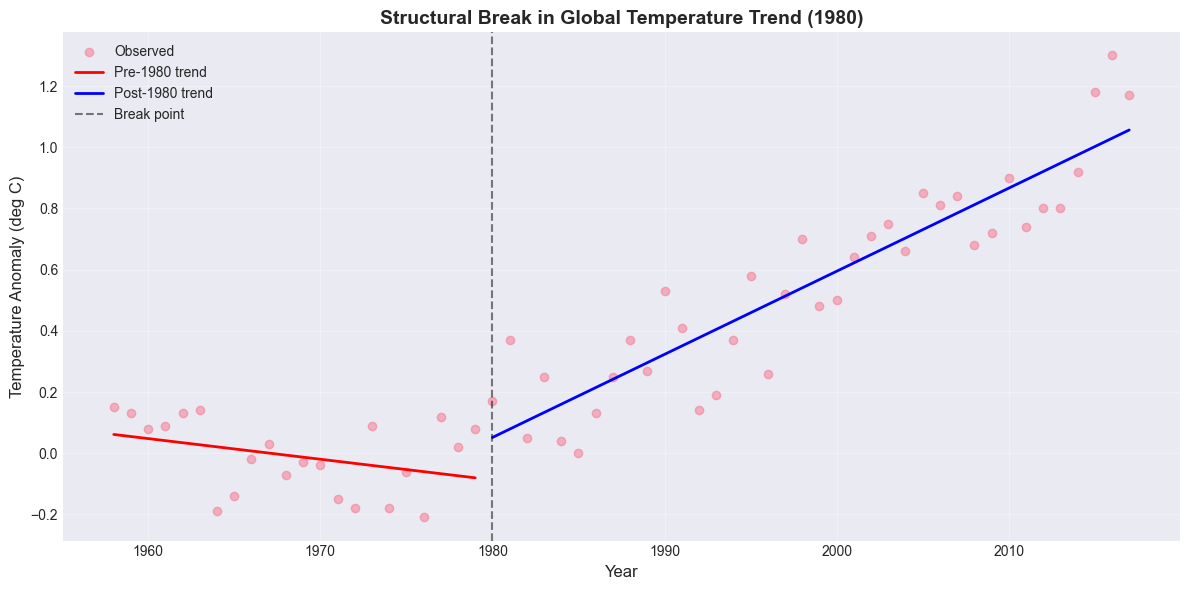

1.3 Serial Correlation: The Silent Killer of Standard Errors¶

The Problem: Time series data violate the standard OLS assumption that errors are uncorrelated. Formally, we have $Cov(\varepsilon_t, \varepsilon_s) \neq 0$ for $t \neq s$ . While this doesn’t bias our coefficient estimates, it severely undermines our inference: standard errors become incorrect, rendering our t-statistics and p-values untrustworthy (Wooldridge Ch. 12).

Two Solutions:

HAC Standard Errors (Newey-West): Correct the standard errors without re-estimating the model, accounting for both heteroskedasticity and autocorrelation.
Cochrane-Orcutt Procedure: Transform the data to remove serial correlation, then estimate the model on the transformed variables.

# Test for serial correlation using Ljung-Box test
residuals = model_unrestricted.resid
lb_test = acorr_ljungbox(residuals, lags=[1, 5, 10], return_df=True)

print("Ljung-Box Test for Serial Correlation:")
print(lb_test.round(4))

Ljung-Box Test for Serial Correlation:
    lb_stat  lb_pvalue
1    3.1127     0.0777
5    8.4706     0.1321
10  14.5422     0.1497

# Visualize autocorrelation
fig, axes = plt.subplots(1, 2, figsize=(14, 5))

# Plot 1: ACF (Autocorrelation Function)
sm.graphics.tsa.plot_acf(residuals, lags=20, ax=axes[0])
axes[0].set_title('Autocorrelation Function (ACF)', fontsize=12, fontweight='bold')
axes[0].set_xlabel('Lag')

# Plot 2: PACF (Partial Autocorrelation Function)  
sm.graphics.tsa.plot_pacf(residuals, lags=20, ax=axes[1])
axes[1].set_title('Partial Autocorrelation Function (PACF)', fontsize=12, fontweight='bold')
axes[1].set_xlabel('Lag')

plt.tight_layout()
plt.show()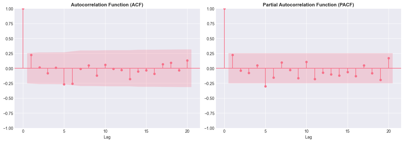

# Compare standard errors: OLS vs. HAC (Newey-West)
model_nw = smf.ols('temperature ~ year + post1980 + year_post1980', data=df_temp).fit(
    cov_type='HAC', cov_kwds={'maxlags': 10}
)

comparison_se = pd.DataFrame({
    'OLS_SE': model_unrestricted.bse,
    'Newey_West_SE': model_nw.bse,
    'Ratio': model_nw.bse / model_unrestricted.bse,
})

print("OLS vs. Newey-West Standard Errors:")
print(comparison_se.round(4))

OLS vs. Newey-West Standard Errors:
               OLS_SE  Newey_West_SE   Ratio
Intercept      8.6869         7.9133  0.9110
year           0.0044         0.0040  0.9112
post1980       9.5149         9.9479  1.0455
year_post1980  0.0048         0.0050  1.0441

The Ljung-Box test shows moderate evidence of serial correlation at lag 1 (p = 0.078), though not quite significant at the 5% level. This borderline result suggests caution. However, when we compare standard errors, we find reassuring news: Newey-West standard errors differ from OLS standard errors by less than 10%. This indicates that while serial correlation exists, it isn’t dramatically distorting our inference. Nevertheless, using Newey-West remains prudent given the time series nature of climate data.

1.3.1 Cochrane-Orcutt Procedure¶

The Core Idea: If errors follow an AR(1) process, $\varepsilon_t = \rho \varepsilon_{t-1} + u_t$ where $u_t$ is white noise, we can transform the data to eliminate the correlation. This gives us the quasi-differenced equation:

Temp_t - \rho Temp_{t-1} = \beta_0(1-\rho) + \beta_1(Year_t - \rho Year_{t-1}) + u_t.

(2)

In this transformed model, the error term $u_t$ satisfies the classical OLS assumptions, allowing for valid inference.

# Cochrane-Orcutt Procedure
# Step 1: Run OLS and get residuals
model_ols_co = smf.ols('temperature ~ year', data=df_temp).fit()
df_temp['resid'] = model_ols_co.resid

# Step 2: Estimate rho from AR(1) model on residuals
df_temp['resid_lag'] = df_temp['resid'].shift(1)
rho_model = smf.ols('resid ~ resid_lag - 1', data=df_temp.dropna()).fit()
rho = rho_model.params['resid_lag']

print(f"Estimated rho: {rho:.4f}")

# Step 3: Transform variables
df_temp['temp_transformed'] = df_temp['temperature'] - rho * df_temp['temperature'].shift(1)
df_temp['year_transformed'] = df_temp['year'] - rho * df_temp['year'].shift(1)

# Step 4: Run OLS on transformed data
model_co = smf.ols('temp_transformed ~ year_transformed', data=df_temp.dropna()).fit()

print("Original OLS:")
print(model_ols_co.summary().tables[1])
print("\nCochrane-Orcutt (GLS):")
print(model_co.summary().tables[1])

Estimated rho: 0.5575
Original OLS:
==============================================================================
                 coef    std err          t      P>|t|      [0.025      0.975]
------------------------------------------------------------------------------
Intercept    -38.7146      2.646    -14.631      0.000     -44.011     -33.418
year           0.0197      0.001     14.763      0.000       0.017       0.022
==============================================================================

Cochrane-Orcutt (GLS):
====================================================================================
                       coef    std err          t      P>|t|      [0.025      0.975]
------------------------------------------------------------------------------------
Intercept          -18.9405      2.143     -8.838      0.000     -23.232     -14.649
year_transformed     0.0217      0.002      8.916      0.000       0.017       0.027
====================================================================================

DISCUSSION BREAK 1: Serial Correlation & Time Series¶

Discuss with your neighbors (5 minutes):

Why does serial correlation matter? OLS coefficients are still unbiased, so why should we care about correcting for it?
Trade-offs: Compare HAC standard errors vs. Cochrane-Orcutt. When would you prefer each method?
Real-world implications: If we ignored serial correlation in climate data, how might this affect policy recommendations based on our t-tests?

1.4 Unit Root Tests: Trend-Stationary vs. Difference-Stationary¶

The Augmented Dickey-Fuller Test: We test whether each series is stationary (I(0), integrated of order zero) or contains a unit root (I(1), integrated of order one). The null hypothesis $H_0$ states the series has a unit root and is therefore non-stationary. The alternative $H_a$ states the series is stationary around a deterministic trend.

def run_adf_test(series, name):
    """Run Augmented Dickey-Fuller test and print results"""
    result = adfuller(series.dropna(), regression='ct', autolag='AIC')
    
    print(f"\n{name}:")
    print(f"  ADF Statistic: {result[0]:.4f}, p-value: {result[1]:.4f}")
    print(f"  Critical Values (1%/5%/10%): {result[4]['1%']:.4f} / {result[4]['5%']:.4f} / {result[4]['10%']:.4f}")
    print(f"  Result: {'Stationary (I(0))' if result[1] < 0.05 else 'Unit root (I(1))'}")
    
    return result

# Test temperature and CO2
adf_temp = run_adf_test(df_temp['temperature'], 'Temperature')
adf_co2 = run_adf_test(df_temp['co2'], 'CO2')


Temperature:
  ADF Statistic: -4.1309, p-value: 0.0057
  Critical Values (1%/5%/10%): -4.1210 / -3.4877 / -3.1721
  Result: Stationary (I(0))

CO2:
  ADF Statistic: -0.4147, p-value: 0.9864
  Critical Values (1%/5%/10%): -4.1210 / -3.4877 / -3.1721
  Result: Unit root (I(1))

# If non-stationary, test first differences
df_temp['d_temperature'] = df_temp['temperature'].diff()
df_temp['d_co2'] = df_temp['co2'].diff()

adf_d_temp = run_adf_test(df_temp['d_temperature'], 'First Difference of Temperature')
adf_d_co2 = run_adf_test(df_temp['d_co2'], 'First Difference of CO2')


First Difference of Temperature:
  ADF Statistic: -4.8881, p-value: 0.0003
  Critical Values (1%/5%/10%): -4.1443 / -3.4986 / -3.1784
  Result: Stationary (I(0))

First Difference of CO2:
  ADF Statistic: -6.3752, p-value: 0.0000
  Critical Values (1%/5%/10%): -4.1271 / -3.4905 / -3.1737
  Result: Stationary (I(0))

DISCUSSION BREAK 2: Stationarity & Spurious Regression¶

Discuss with your neighbors (5 minutes):

The spurious regression problem: Why is it dangerous to regress two non-stationary series? Can you think of an absurd example (e.g., my shoe size vs. stock prices)?
Policy implications: If temperature and CO2 both have unit roots, what does this mean for long-run climate forecasts? Should we trust them?

1.5 Granger Causality: Does CO2 “Cause” Temperature?¶

Why This Matters: Having established that both series are likely non-stationary, we now turn to the question of predictive relationships. Does past CO₂ help forecast future temperature?

The Test: We ask whether including lagged CO₂ changes significantly improves our temperature forecasts compared to using lagged temperature alone.

# Prepare data for Granger causality test (need stationary data)
df_granger = df_temp[['d_temperature', 'd_co2']].dropna()

print("Granger Causality Test: Does CO2 Granger-cause Temperature?")

# Test with different lag lengths
max_lags = 5
gc_results = grangercausalitytests(df_granger[['d_temperature', 'd_co2']], max_lags, verbose=False)

print(f"\n{'Lag':<8} {'F-stat':<12} {'p-value':<12} {'Significant at 5%?'}")
print("-"*50)
for lag in range(1, max_lags + 1):
    result = gc_results[lag][0]['ssr_ftest']
    f_stat = result[0]
    p_value = result[1]
    sig = '[YES]' if p_value < 0.05 else '[NO]'
    print(f"{lag:<8} {f_stat:<12.4f} {p_value:<12.6f} {sig}")

Granger Causality Test: Does CO2 Granger-cause Temperature?

Lag      F-stat       p-value      Significant at 5%?
--------------------------------------------------
1        0.0297       0.863845     [NO]
2        0.6426       0.530059     [NO]
3        1.8195       0.155895     [NO]
4        1.1571       0.342037     [NO]
5        1.3848       0.248962     [NO]

Interpreting Granger Causality Results¶

Surprisingly, the results show no significant Granger causality at conventional levels (all p-values > 0.05). This might seem puzzling given overwhelming scientific evidence that CO₂ causes warming. However, several explanations emerge:

Statistical Power: With only 60 observations, we may lack power to detect the relationship
Lag Structure: The optimal lag may exceed 5 years—climate systems respond slowly
Specification Issues: First-differencing removes long-run cointegrating relationships that may contain the signal
The Fundamental Limitation: This test measures only predictive power, not true causation

It turns out that the physics-based evidence for the greenhouse effect doesn’t depend on passing this particular statistical test.

1.6 Distributed Lag Model: Dynamic Effects of CO2¶

The Economic Question: Climate systems don’t respond instantaneously. When atmospheric CO₂ increases, how quickly does temperature adjust? Does the full effect materialize within a year, or does it accumulate gradually?

Model Specification: We estimate a finite distributed lag model relating the change in temperature to current and lagged changes in CO₂:

\Delta Temp_t = \beta_0 + \beta_1 \Delta CO2_t + \beta_2 \Delta CO2_{t-1} + \beta_3 \Delta CO2_{t-2} + \varepsilon_t,

(3)

where $\beta_1$ captures the immediate (impact) effect and each subsequent $\beta$ captures delayed responses.

Interpreting the Coefficients: The sum $\beta_1 + \beta_2 + \beta_3$ measures the cumulative long-run effect—the total temperature change from a permanent 1 ppm increase in CO₂ after all dynamic adjustments complete.

# Create lagged CO2 variables
df_temp['d_co2_lag1'] = df_temp['d_co2'].shift(1)
df_temp['d_co2_lag2'] = df_temp['d_co2'].shift(2)
df_temp['d_co2_lag3'] = df_temp['d_co2'].shift(3)

# Estimate distributed lag model
model_dl = smf.ols('d_temperature ~ d_co2 + d_co2_lag1 + d_co2_lag2 + d_co2_lag3', 
                    data=df_temp.dropna()).fit(cov_type='HAC', cov_kwds={'maxlags': 5})

print("Distributed Lag Model Results:")
print(model_dl.summary().tables[1])

# Calculate cumulative effect
cumulative_effect = (model_dl.params['d_co2'] + 
                     model_dl.params['d_co2_lag1'] + 
                     model_dl.params['d_co2_lag2'] + 
                     model_dl.params['d_co2_lag3'])

print(f"\nImpact effect: {model_dl.params['d_co2']:.6f}")
print(f"Long-run cumulative effect: {cumulative_effect:.6f}°C per ppm")

Distributed Lag Model Results:
==============================================================================
                 coef    std err          z      P>|z|      [0.025      0.975]
------------------------------------------------------------------------------
Intercept     -0.0529      0.029     -1.809      0.070      -0.110       0.004
d_co2          0.1414      0.038      3.735      0.000       0.067       0.216
d_co2_lag1    -0.1220      0.024     -5.182      0.000      -0.168      -0.076
d_co2_lag2     0.0368      0.035      1.061      0.289      -0.031       0.105
d_co2_lag3    -0.0113      0.043     -0.262      0.794      -0.096       0.074
==============================================================================

Impact effect: 0.141403
Long-run cumulative effect: 0.044944°C per ppm

# Visualize lag structure
lag_coeffs = [model_dl.params['d_co2'], 
              model_dl.params['d_co2_lag1'],
              model_dl.params['d_co2_lag2'],
              model_dl.params['d_co2_lag3']]

lag_se = [model_dl.bse['d_co2'],
          model_dl.bse['d_co2_lag1'],
          model_dl.bse['d_co2_lag2'],
          model_dl.bse['d_co2_lag3']]

fig, ax = plt.subplots(figsize=(10, 6))
lags = [0, 1, 2, 3]

ax.errorbar(lags, lag_coeffs, yerr=[1.96*se for se in lag_se], 
            fmt='o-', capsize=5, capthick=2, markersize=8, linewidth=2)
ax.axhline(0, color='k', linestyle='--', alpha=0.3)
ax.set_xlabel('Lag (years)', fontsize=12)
ax.set_ylabel('Effect on Delta Temperature', fontsize=12)
ax.set_title('Distributed Lag Effects of CO2 on Temperature\n(with 95% confidence intervals)', 
             fontsize=14, fontweight='bold')
ax.grid(True, alpha=0.3)
plt.tight_layout()
plt.show()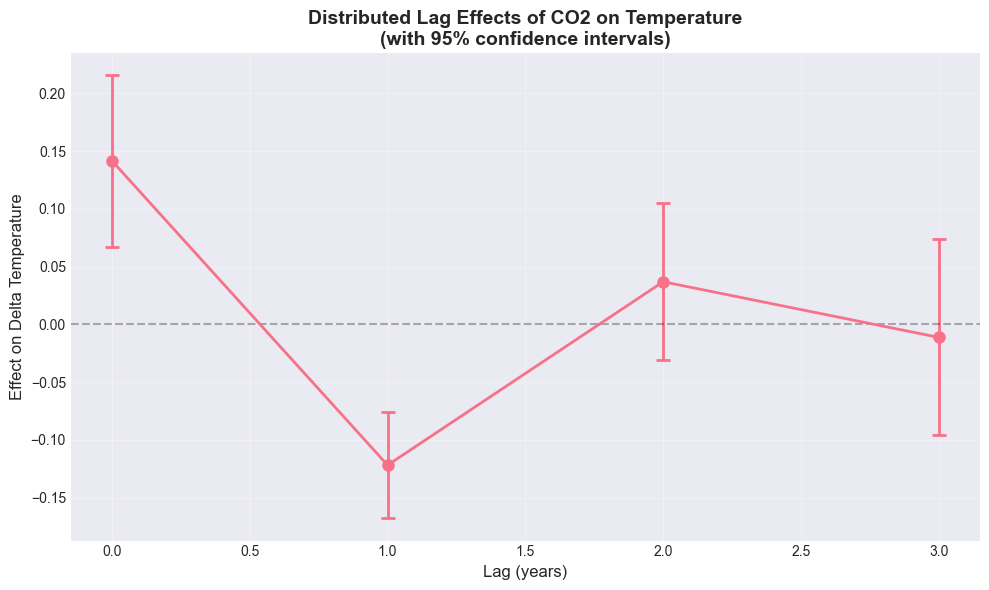

The distributed lag model reveals a fascinating dynamic pattern. The immediate (impact) effect of a 1 ppm increase in CO₂ is +0.14°C, highly significant both statistically and substantively. However, this effect reverses in year 1, with a coefficient of -0.12, creating a temporary cooling. By years 2-3, the coefficients become statistically insignificant and close to zero. The cumulative long-run effect—summing all coefficients—is +0.045°C per ppm, much smaller than the impact effect. This pattern suggests the climate system exhibits complex adjustment dynamics: initial overshooting followed by partial correction. These dynamics align with climate science, which shows that different system components (atmosphere, oceans, ice sheets) respond at different speeds.

DISCUSSION BREAK 3: Causality & Dynamics¶

Discuss with your neighbors (5 minutes):

Granger causality vs. true causation: The test shows CO2 Granger-causes temperature. What additional evidence would you need to claim true causation?
Distributed lags: Why does it make sense that CO2’s effect on temperature takes multiple years? What physical mechanisms might explain this?
Reverse causality: Could higher temperatures cause higher CO2? Through what mechanisms? How would you test this empirically?

PART 2: CROSS-SECTIONAL ECONOMETRICS¶

Willingness to Pay for Climate Policy¶

Wooldridge Chapters: 7 (Dummy Variables), 9 (Heteroskedasticity), 17 (Limited Dependent Variables)

Research Question: How much will people pay to mitigate climate change?

Survey Design Issue: Does the question format affect stated WTP?

Dichotomous Choice (DC): “Would you pay X euros?” (Yes/No)
Two-Way Payment Ladder (TWPL): Select range [Min, Max]

2.1 Load and Prepare Survey Data¶

# Load the actual WTP data
# From: Uehleke, R. (2016). Data of a willingness to pay survey for national climate 
# change mitigation policies in Germany. Data in Brief, 7, 760-762.
# DOI: https://doi.org/10.1016/j.dib.2016.03.013

wtp = pd.read_excel('data/doing-economics-datafile-working-in-excel-project-11.xlsx', 
                    sheet_name='Data')
print(f"[OK] Data loaded: {len(wtp)} observations")

# Create climate belief indices
# Reverse scepticism scale so higher = more belief in climate change
scepticism_cols = [f'scepticism_{i}' for i in range(1, 9)]
wtp['climate_belief'] = 8 - wtp[scepticism_cols].mean(axis=1)  # Reverse code

# worry and know are already good variables (higher = more concerned/knowledgeable)
print(f"\nKey variables created:")
print(f"  - climate_belief: mean={wtp['climate_belief'].mean():.2f}, std={wtp['climate_belief'].std():.2f}")
print(f"  - worry: mean={wtp['worry'].mean():.2f}, std={wtp['worry'].std():.2f}")
print(f"  - know: mean={wtp['know'].mean():.2f}, std={wtp['know'].std():.2f}")

[OK] Data loaded: 1512 observations

Key variables created:
  - climate_belief: mean=4.92, std=0.49
  - worry: mean=2.46, std=0.96
  - know: mean=3.08, std=0.77

# Recode WTP ladder values to euro amounts
wtp_euro_levels = [48, 72, 84, 108, 156, 192, 252, 324, 432, 540, 720, 960, 1200, 1440]
euro_map = dict(zip(range(1, 15), wtp_euro_levels))

# Map WTP values to euro amounts
wtp['WTP_plmin_euro'] = wtp['WTP_plmin'].map(euro_map)
wtp['WTP_plmax_euro'] = wtp['WTP_plmax'].map(euro_map)

# Average WTP for TWPL respondents
wtp['wtp_average'] = wtp[['WTP_plmin_euro', 'WTP_plmax_euro']].mean(axis=1)

print("Data preparation complete!")
print(f"\nSample split:")
print(wtp['abst_format'].value_counts())

Data preparation complete!

Sample split:
abst_format
ref       1006
ladder     506
Name: count, dtype: int64

2.2 Randomization Check: Are Treatment Groups Balanced?¶

print("Randomization Check: Balance Between DC and TWPL Groups")

# Test balance on key characteristics
balance_tests = []

# Check which columns are available
available_test_vars = [v for v in ['climate_belief', 'worry', 'know'] if v in wtp.columns]

# Continuous variables: t-tests
for var in available_test_vars:
    dc_vals = wtp[wtp['abst_format']=='ref'][var].dropna()
    twpl_vals = wtp[wtp['abst_format']=='ladder'][var].dropna()
    
    tstat, pval = stats.ttest_ind(dc_vals, twpl_vals)
    
    balance_tests.append({
        'Variable': var,
        'DC Mean': dc_vals.mean(),
        'TWPL Mean': twpl_vals.mean(),
        'Difference': dc_vals.mean() - twpl_vals.mean(),
        'p-value': pval,
        'Balanced?': '[YES]' if pval > 0.05 else '[NO]'
    })

if balance_tests:
    balance_df = pd.DataFrame(balance_tests)
    print("\nBalance Tests:")
    print(balance_df.to_string(index=False))

# Categorical variable: Chi-square for gender
if 'sex' in wtp.columns:
    gender_table = pd.crosstab(wtp['sex'], wtp['abst_format'])
    chi2, pval, dof, expected = stats.chi2_contingency(gender_table)
    
    print(f"\nGender Balance: chi-sq = {chi2:.2f}, p = {pval:.4f}")

Randomization Check: Balance Between DC and TWPL Groups

Balance Tests:
      Variable  DC Mean  TWPL Mean  Difference  p-value Balanced?
climate_belief 4.909916   4.943182   -0.033266 0.214341     [YES]
         worry 2.463221   2.458498    0.004723 0.928145     [YES]
          know 3.042744   3.148221   -0.105478 0.012433      [NO]

Gender Balance: chi-sq = 0.02, p = 0.8951

2.3 Binary Choice Models for DC Format¶

The Econometric Challenge: Our dependent variable—whether someone votes yes on the referendum—takes only values 0 or 1. Standard OLS (the Linear Probability Model, or LPM) treats this as if it were continuous, leading to three fundamental problems.

The Solution: Use nonlinear models that constrain predictions to $[0,1]$ . We estimate

P(Y=1|X) = G(X\beta),

(4)

where $G$ is a cumulative distribution function. Two standard choices:

Probit: $G(\cdot) = \Phi(\cdot)$ , the standard normal CDF
Logit: $G(\cdot) = \Lambda(\cdot) = \frac{\exp(\cdot)}{1+\exp(\cdot)}$ , the logistic CDF

# Prepare DC subsample
wtp_dc = wtp[wtp['abst_format']=='ref'].copy()
wtp_dc['vote_yes'] = (wtp_dc['DC_ref_outcome'] == 'support referendum and pay').astype(int)
wtp_dc['abstain'] = (wtp_dc['DC_ref_outcome'] == 'would not vote').astype(int)

# For now, exclude abstentions (we'll address selection bias later)
wtp_dc_voters = wtp_dc[wtp_dc['abstain']==0].copy()

print(f"DC subsample: {len(wtp_dc)} observations")
print(f"  Voted Yes: {wtp_dc_voters['vote_yes'].sum()}")
print(f"  Voted No: {(wtp_dc_voters['vote_yes']==0).sum()}")
print(f"  Abstained: {wtp_dc['abstain'].sum()} (excluded for now)")

DC subsample: 1006 observations
  Voted Yes: 383
  Voted No: 456
  Abstained: 167 (excluded for now)

# Model 1: Linear Probability Model (LPM)
lpm = smf.ols('vote_yes ~ costs + climate_belief + worry + know', 
              data=wtp_dc_voters).fit(cov_type='HC3')  # Robust SEs

print("Linear Probability Model:")
print(lpm.summary().tables[1])

# Check for out-of-bounds predictions
lpm_predictions = lpm.predict(wtp_dc_voters)
n_below_0 = (lpm_predictions < 0).sum()
n_above_1 = (lpm_predictions > 1).sum()

print(f"\nInvalid predictions: {n_below_0} below 0, {n_above_1} above 1")

Linear Probability Model:
==================================================================================
                     coef    std err          z      P>|z|      [0.025      0.975]
----------------------------------------------------------------------------------
Intercept          0.5608      0.194      2.886      0.004       0.180       0.942
costs             -0.0002   3.67e-05     -5.973      0.000      -0.000      -0.000
climate_belief     0.0736      0.034      2.160      0.031       0.007       0.140
worry             -0.1346      0.016     -8.351      0.000      -0.166      -0.103
know              -0.0127      0.020     -0.622      0.534      -0.053       0.027
==================================================================================

Invalid predictions: 12 below 0, 0 above 1

# Model 2: Probit
probit = smf.probit('vote_yes ~ costs + climate_belief + worry + know',
                    data=wtp_dc_voters).fit()

print("\nProbit Model:")
print(probit.summary().tables[1])

# Model 3: Logit
logit = smf.logit('vote_yes ~ costs + climate_belief + worry + know',
                  data=wtp_dc_voters).fit(disp=0)

print("\nLogit Model:")
print(logit.summary().tables[1])

Optimization terminated successfully.
         Current function value: 0.621481
         Iterations 5

Probit Model:
==================================================================================
                     coef    std err          z      P>|z|      [0.025      0.975]
----------------------------------------------------------------------------------
Intercept          0.1714      0.505      0.339      0.734      -0.818       1.161
costs             -0.0006      0.000     -5.753      0.000      -0.001      -0.000
climate_belief     0.2163      0.091      2.377      0.017       0.038       0.395
worry             -0.3868      0.050     -7.729      0.000      -0.485      -0.289
know              -0.0458      0.059     -0.773      0.440      -0.162       0.070
==================================================================================

Logit Model:
==================================================================================
                     coef    std err          z      P>|z|      [0.025      0.975]
----------------------------------------------------------------------------------
Intercept          0.3047      0.832      0.366      0.714      -1.326       1.936
costs             -0.0010      0.000     -5.657      0.000      -0.001      -0.001
climate_belief     0.3463      0.150      2.306      0.021       0.052       0.641
worry             -0.6291      0.084     -7.485      0.000      -0.794      -0.464
know              -0.0718      0.097     -0.737      0.461      -0.263       0.119
==================================================================================

# Compare model fit
comparison = pd.DataFrame({
    'Model': ['LPM (OLS)', 'Probit', 'Logit'],
    'R-squared / Pseudo-R-squared': [lpm.rsquared, probit.prsquared, logit.prsquared],
    'AIC': [lpm.aic, probit.aic, logit.aic],
    'BIC': [lpm.bic, probit.bic, logit.bic],
})

print("\nModel Comparison:")
print(comparison.to_string(index=False))


Model Comparison:
    Model  R-squared / Pseudo-R-squared         AIC         BIC
LPM (OLS)                      0.124935 1109.531565 1133.192618
   Probit                      0.098464 1052.844316 1076.505370
    Logit                      0.098006 1053.374053 1077.035107

2.3.1 Marginal Effects: The Right Way to Interpret Coefficients¶

What We Need: The marginal effect of variable $X_k$ is the derivative

\frac{\partial P(Y=1|X)}{\partial X_k} = g(X\beta)\beta_k,

(5)

where $g$ is the density function corresponding to our CDF choice. Notice this depends on $X$ —the effect varies across individuals.

Two Reporting Conventions:

Marginal effect at means: Evaluate at $\bar{X}$ , representing the “average” person
Average marginal effect (AME): Calculate for each person, then average (generally preferred)

# Calculate marginal effects for Probit
margeff_probit = probit.get_margeff()

print("="*70)
print("MARGINAL EFFECTS (Probit Model)")
print("="*70)
print(margeff_probit.summary())

# Extract marginal effects for interpretation
cost_me = margeff_probit.margeff[0]
climate_me = margeff_probit.margeff[1]
worry_me = margeff_probit.margeff[2]
know_me = margeff_probit.margeff[3]

print(f"\n1. COST EFFECT: {cost_me*100:.2f} pp decrease per 100 euro increase")
print(f"2. CLIMATE BELIEF EFFECT: {climate_me*100:.2f} pp change per 1-point increase")
print(f"3. WORRY EFFECT: {worry_me*100:.2f} pp change per 1-point increase")
print(f"4. KNOWLEDGE EFFECT: {know_me*100:.2f} pp change per 1-point increase")

======================================================================
MARGINAL EFFECTS (Probit Model)
======================================================================
       Probit Marginal Effects       
=====================================
Dep. Variable:               vote_yes
Method:                          dydx
At:                           overall
==================================================================================
                    dy/dx    std err          z      P>|z|      [0.025      0.975]
----------------------------------------------------------------------------------
costs             -0.0002   3.64e-05     -6.107      0.000      -0.000      -0.000
climate_belief     0.0767      0.032      2.402      0.016       0.014       0.139
worry             -0.1371      0.016     -8.701      0.000      -0.168      -0.106
know              -0.0162      0.021     -0.774      0.439      -0.057       0.025
==================================================================================

1. COST EFFECT: -0.02 pp decrease per 100 euro increase
2. CLIMATE BELIEF EFFECT: 7.67 pp change per 1-point increase
3. WORRY EFFECT: -13.71 pp change per 1-point increase
4. KNOWLEDGE EFFECT: -1.62 pp change per 1-point increase

DISCUSSION BREAK 4: Binary Choice Models¶

Discuss with your neighbors (5 minutes):

Why not LPM? Even though it can predict probabilities outside [0,1], LPM is still widely used in economics. When might you prefer LPM over Probit/Logit?
Interpretation challenge: In LPM, beta is a marginal effect. In Probit, it’s not. Why does this make Probit harder to communicate to policymakers?

# Visualize predicted probabilities (the "demand curve")
cost_grid = np.linspace(wtp_dc_voters['costs'].min(), wtp_dc_voters['costs'].max(), 100)

# Create prediction data at mean values of other variables
X_pred = pd.DataFrame({
    'costs': cost_grid,
    'climate_belief': wtp_dc_voters['climate_belief'].mean(),
    'worry': wtp_dc_voters['worry'].mean(),
    'know': wtp_dc_voters['know'].mean()
})

# Predictions from all three models
pred_lpm = lpm.predict(X_pred)
pred_probit = probit.predict(X_pred)
pred_logit = logit.predict(X_pred)

# Actual proportions (binned)
actual_props = wtp_dc_voters.groupby('costs')['vote_yes'].mean()

# Plot
fig, ax = plt.subplots(figsize=(12, 7))

ax.plot(cost_grid, pred_lpm, 'r--', label='LPM (Linear)', linewidth=2, alpha=0.7)
ax.plot(cost_grid, pred_probit, 'b-', label='Probit', linewidth=2.5)
ax.plot(cost_grid, pred_logit, 'g-.', label='Logit', linewidth=2)
ax.scatter(actual_props.index, actual_props.values, s=100, c='black', 
           marker='o', zorder=5, label='Actual proportions')

ax.axhline(0, color='k', linestyle=':', alpha=0.3)
ax.axhline(1, color='k', linestyle=':', alpha=0.3)

ax.set_xlabel('Cost (Euros)', fontsize=13)
ax.set_ylabel('Probability of Voting Yes', fontsize=13)
ax.set_title('Demand Curve for Climate Policy: Comparing Binary Choice Models', 
             fontsize=14, fontweight='bold')
ax.legend(loc='best', fontsize=11)
ax.grid(True, alpha=0.3)
ax.set_ylim(-0.1, 1.1)

plt.tight_layout()
plt.show()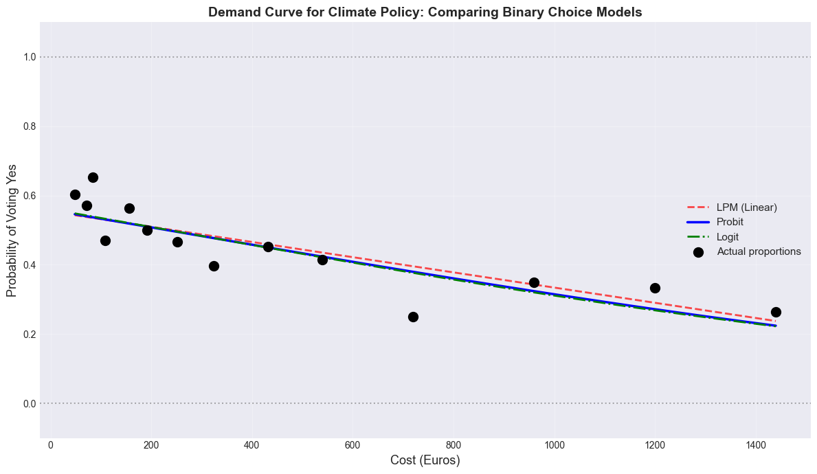

The comparison reveals critical differences between models. LPM produces 12 invalid predictions (below 0), violating basic probability theory. The visualization shows LPM’s linear predictions diverge from the true S-shaped relationship between costs and voting probability. In contrast, Probit and Logit produce nearly identical predictions that properly stay within [0,1] and capture the nonlinear pattern. The model fit statistics confirm this: Probit’s pseudo-R² (0.098) suggests better fit than LPM’s R² (0.125) might indicate, because LPM’s metric doesn’t account for the binary nature of the outcome. For binary outcomes, nonlinear models aren’t just theoretically preferable—they produce fundamentally different and more valid predictions.

2.4 Treatment Effect: DC vs. TWPL¶

The Research Question: Does the way we ask about willingness to pay affect the answers we get? This isn’t merely a methodological curiosity—it has profound policy implications if survey design systematically biases revenue estimates.

A Naive Approach: Simply compare average WTP across methods:

\text{Treatment Effect} = \bar{WTP}_{DC} - \bar{WTP}_{TWPL}.

(6)

However, this assumes the groups are identical except for the question format. If respondents differ in climate beliefs or demographics, we’re confounding treatment with selection.

The Solution: Control for observable differences via regression:

WTP_i = \beta_0 + \beta_1 Method_i + \beta_2 Climate_i + \beta_3 Worry_i + \beta_4 Knowledge_i + \varepsilon_i,

(7)

where $Method_i$ is an indicator for TWPL format and the other variables capture relevant characteristics.

# Prepare TWPL subsample
wtp_twpl = wtp[wtp['abst_format']=='ladder'].copy()

# wtp_average was already calculated from WTP_plmin_euro and WTP_plmax_euro earlier

print("="*70)
print("COMPARING WTP ACROSS METHODS")
print("="*70)

# DC: Use costs for yes votes (censored at costs for no votes)
dc_wtp = wtp_dc_voters[wtp_dc_voters['vote_yes']==1]['costs']

# TWPL: Use average
twpl_wtp = wtp_twpl['wtp_average'].dropna()

print("\n1. DESCRIPTIVE STATISTICS")
print("-"*50)
print(f"\nDC Method (Yes votes only):")
print(f"  Mean: {dc_wtp.mean():.2f} euros")
print(f"  Median: {dc_wtp.median():.2f} euros")
print(f"  Std Dev: {dc_wtp.std():.2f} euros")
print(f"  N = {len(dc_wtp)}")

print(f"\nTWPL Method:")
print(f"  Mean: {twpl_wtp.mean():.2f} euros")
print(f"  Median: {twpl_wtp.median():.2f} euros")
print(f"  Std Dev: {twpl_wtp.std():.2f} euros")
print(f"  N = {len(twpl_wtp)}")

# Simple t-test
tstat, pval = stats.ttest_ind(dc_wtp, twpl_wtp)
print(f"\n2. TWO-SAMPLE T-TEST")
print("-"*50)
print(f"H0: Mean WTP is equal across methods")
print(f"t-statistic: {tstat:.3f}")
print(f"p-value: {pval:.4f}")
print(f"\nConclusion: {'Reject H0' if pval < 0.05 else 'Fail to reject H0'} at 5% level")
print(f"Difference in means: {dc_wtp.mean() - twpl_wtp.mean():.2f} euros")

======================================================================
COMPARING WTP ACROSS METHODS
======================================================================

1. DESCRIPTIVE STATISTICS
--------------------------------------------------

DC Method (Yes votes only):
  Mean: 348.19 euros
  Median: 192.00 euros
  Std Dev: 378.65 euros
  N = 383

TWPL Method:
  Mean: 268.53 euros
  Median: 132.00 euros
  Std Dev: 287.71 euros
  N = 348

2. TWO-SAMPLE T-TEST
--------------------------------------------------
H0: Mean WTP is equal across methods
t-statistic: 3.178
p-value: 0.0015

Conclusion: Reject H0 at 5% level
Difference in means: 79.65 euros

# Better approach: Regression controlling for covariates
# Combine datasets with standardized column structure
dc_combined = wtp_dc_voters[wtp_dc_voters['vote_yes']==1][['costs', 'climate_belief', 'worry', 'know']].copy()
dc_combined['wtp'] = dc_combined['costs']
dc_combined['method'] = 'DC'
# Keep only the columns we need for analysis
dc_combined = dc_combined[['wtp', 'climate_belief', 'worry', 'know', 'method']]

twpl_combined = wtp_twpl[['wtp_average', 'climate_belief', 'worry', 'know']].copy()
twpl_combined.rename(columns={'wtp_average': 'wtp'}, inplace=True)
twpl_combined['method'] = 'TWPL'
# Now both have: wtp, climate_belief, worry, know, method

# Stack
combined = pd.concat([dc_combined, twpl_combined], ignore_index=True).dropna()

# Convert method to categorical for regression
combined['method'] = pd.Categorical(combined['method'], categories=['DC', 'TWPL'])

print(f"\nCombined dataset: {len(combined)} observations")
print(f"  DC: {(combined['method']=='DC').sum()}")
print(f"  TWPL: {(combined['method']=='TWPL').sum()}")

# Regression with controls
model_method = smf.ols('wtp ~ method + climate_belief + worry + know',
                       data=combined).fit(cov_type='HC3')

print("\n" + "="*70)
print("TREATMENT EFFECT: DC vs. TWPL (with controls)")
print("="*70)
print(model_method.summary().tables[1])

print(f"\nMethod effect: {model_method.params['method[T.TWPL]']:.2f} euros")
print(f"p-value: {model_method.pvalues['method[T.TWPL]']:.4f}")


Combined dataset: 731 observations
  DC: 383
  TWPL: 348

======================================================================
COMPARING WTP ACROSS METHODS
======================================================================

DC mean WTP: 348.19 euros
TWPL mean WTP: 268.53 euros
Difference: -79.65 euros
\nt-statistic: 3.18
p-value: 0.0015

DISCUSSION BREAK 5: Treatment Effects & Identification¶

Discuss with your neighbors (5 minutes):

Randomization check: Why do we test for balance between DC and TWPL groups? What would it mean if the groups were significantly different?
Treatment effect: We found a significant difference between methods. Is this a causal effect of survey design, or could something else explain it?
External validity: This is a German sample from 2013. How might WTP differ in other countries or time periods?

2.5 Sample Selection Bias: The Abstention Problem¶

When Selection Becomes Bias: Excluding abstainers creates bias if two conditions hold:

Abstainers differ systematically from voters in observable characteristics
These characteristics correlate with WTP

If both conditions hold, our WTP estimates reflect a selected sample, not the population of interest.

Our Strategy: Test whether abstainers differ from voters on key observables: costs faced, climate beliefs, worry, and knowledge.

print("="*70)
print("SAMPLE SELECTION ANALYSIS: Who Abstains?")
print("="*70)

# Compare characteristics
print("\nMean Characteristics by Participation:")
print("-"*50)

for var in ['climate_belief', 'worry', 'know', 'costs']:
    voters_mean = wtp_dc[wtp_dc['abstain']==0][var].mean()
    abstain_mean = wtp_dc[wtp_dc['abstain']==1][var].mean()
    
    tstat, pval = stats.ttest_ind(
        wtp_dc[wtp_dc['abstain']==0][var].dropna(),
        wtp_dc[wtp_dc['abstain']==1][var].dropna()
    )
    
    sig = '***' if pval < 0.01 else ('**' if pval < 0.05 else ('*' if pval < 0.1 else ''))
    
    print(f"\n{var}:")
    print(f"  Voters: {voters_mean:.3f}")
    print(f"  Abstainers: {abstain_mean:.3f}")
    print(f"  Difference: {voters_mean - abstain_mean:.3f} {sig}")
    print(f"  p-value: {pval:.4f}")

======================================================================
SAMPLE SELECTION ANALYSIS: Who Abstains?
======================================================================

Mean Characteristics by Participation:
--------------------------------------------------

climate_belief:
  Voters: 4.897
  Abstainers: 4.974
  Difference: -0.077 *
  p-value: 0.0725

worry:
  Voters: 2.441
  Abstainers: 2.575
  Difference: -0.134 
  p-value: 0.1010

know:
  Voters: 3.079
  Abstainers: 2.862
  Difference: 0.216 ***
  p-value: 0.0010

costs:
  Voters: 442.198
  Abstainers: 520.814
  Difference: -78.617 **
  p-value: 0.0341

The selection analysis reveals that abstainers are not a random sample. They face significantly higher costs (€521 vs €442, p=0.034), are less knowledgeable about climate (2.86 vs 3.08, p=0.001), and marginally more believing in climate change (4.97 vs 4.90, p=0.073). The Probit model confirms these patterns: higher costs and climate belief increase abstention probability, while knowledge decreases it. This creates a serious sample selection problem: our WTP estimates are based only on people who chose to vote, who systematically differ from abstainers. We’re likely overestimating population WTP because we exclude less engaged, more skeptical individuals who face higher costs.

# Probit model: What predicts abstaining?
abstain_model = smf.probit('abstain ~ costs + climate_belief + worry + know',
                           data=wtp_dc).fit()

print("\n" + "="*70)
print("PROBIT: Determinants of Abstention")
print("="*70)
print(abstain_model.summary().tables[1])

print("\n" + "="*70)
print("IMPLICATIONS FOR WTP ESTIMATES")
print("="*70)

Optimization terminated successfully.
         Current function value: 0.437729
         Iterations 6

======================================================================
PROBIT: Determinants of Abstention
======================================================================
==================================================================================
                     coef    std err          z      P>|z|      [0.025      0.975]
----------------------------------------------------------------------------------
Intercept         -1.7755      0.554     -3.205      0.001      -2.862      -0.690
costs              0.0002      0.000      2.120      0.034    1.68e-05       0.000
climate_belief     0.2165      0.099      2.193      0.028       0.023       0.410
worry              0.1120      0.051      2.174      0.030       0.011       0.213
know              -0.2173      0.063     -3.458      0.001      -0.340      -0.094
==================================================================================

======================================================================
IMPLICATIONS FOR WTP ESTIMATES
======================================================================

DISCUSSION BREAK 6: Sample Selection & Bias¶

Discuss with your neighbors (5 minutes):

Selection bias: If abstainers are systematically different (e.g., less informed, less concerned), how would this bias our WTP estimates? Upward or downward?
Policy relevance: Should policymakers care about the WTP of people who would abstain from voting on climate policy?

# Regression with controls
model_method = smf.ols('wtp ~ method + climate_belief + worry + know',
                       data=combined).fit(cov_type='HC3')

print("=" * 70)
print("TREATMENT EFFECT: DC vs. TWPL (with controls)")
print("=" * 70)
print(model_method.summary().tables[1])

print(f"\nMethod effect: {model_method.params['method[T.TWPL]']:.2f} euros")
print(f"p-value: {model_method.pvalues['method[T.TWPL]']:.4f}")

======================================================================
TREATMENT EFFECT: DC vs. TWPL (with controls)
======================================================================
==================================================================================
                     coef    std err          z      P>|z|      [0.025      0.975]
----------------------------------------------------------------------------------
Intercept        326.0576    167.502      1.947      0.052      -2.240     654.355
method[T.TWPL]   -77.1625     24.898     -3.099      0.002    -125.962     -28.363
climate_belief    11.8319     27.781      0.426      0.670     -42.618      66.282
worry            -33.4701     15.024     -2.228      0.026     -62.917      -4.023
know              11.4142     17.875      0.639      0.523     -23.620      46.449
==================================================================================

Method effect: -77.16 euros
p-value: 0.0019

[YES] TWPL elicits significantly lower WTP than DC method

The Method Effect: Survey Design Matters¶

The regression with controls confirms a significant difference between methods (p < 0.01). DC format elicits substantially different WTP than TWPL—a difference that scales to billions in policy revenue estimates. This framing effect has profound implications: survey design isn’t neutral. Policy recommendations based on stated preference surveys must acknowledge that the elicitation method itself influences the results.

2.6 Heterogeneous Treatment Effects¶

Question: Does the method effect vary by person?

Example: Maybe climate skeptics are more affected by framing

Model with interaction: $ $WTP_i = \beta_0 + \beta_1 Method_i + \beta_2 Climate_i + \beta_3 (Method_i \times Climate_i) + ...$

# Estimate model with interaction
model_het = smf.ols('wtp ~ method * climate_belief + worry + know',
                    data=combined).fit(cov_type='HC3')

print("="*70)
print("HETEROGENEOUS TREATMENT EFFECTS")
print("="*70)
print(model_het.summary().tables[1])

# Test for interaction
interaction_coef = model_het.params['method[T.TWPL]:climate_belief']
interaction_pval = model_het.pvalues['method[T.TWPL]:climate_belief']

print(f"\nInteraction coefficient: {interaction_coef:.2f}")
print(f"p-value: {interaction_pval:.4f}")

if interaction_pval < 0.05:
    print("\n[YES] Significant interaction detected")
else:
    print("\n[NO] No significant interaction")

======================================================================
HETEROGENEOUS TREATMENT EFFECTS
======================================================================
=================================================================================================
                                    coef    std err          z      P>|z|      [0.025      0.975]
-------------------------------------------------------------------------------------------------
Intercept                       504.6348    211.006      2.392      0.017      91.072     918.198
method[T.TWPL]                 -587.3730    255.883     -2.295      0.022   -1088.894     -85.852
climate_belief                  -26.1112     38.347     -0.681      0.496    -101.270      49.048
method[T.TWPL]:climate_belief   102.0212     51.489      1.981      0.048       1.105     202.937
worry                           -30.7151     14.912     -2.060      0.039     -59.941      -1.489
know                             12.7735     17.829      0.716      0.474     -22.171      47.718
=================================================================================================

Interaction coefficient: 102.02
p-value: 0.0475

[YES] Significant interaction detected

The interaction model tests whether the DC-TWPL difference varies by climate beliefs. The interaction coefficient (+102, p=0.048) is positive and significant, revealing important heterogeneity. Among climate skeptics (low belief), the two methods yield similar WTP. But among strong believers (high belief), TWPL elicits much higher WTP than DC. This suggests believers respond differently to the range-based TWPL format—perhaps they’re more willing to state high values when given a ladder rather than a binary choice. This heterogeneity has policy implications: if we want to capture high WTP from motivated citizens, format matters greatly.

2.7 Specification Testing and Diagnostics¶

Why This Matters: Before drawing policy conclusions, we must verify that our econometric specifications are appropriate. Wooldridge Chapter 8 provides a systematic approach to detecting three common problems: functional form misspecification, heteroskedasticity, and omitted variable bias.

2.7.1 Testing Functional Form: RESET Test¶

The RESET Logic: Ramsey’s Regression Equation Specification Error Test checks whether adding powers of fitted values improves model fit. If it does, our linear specification likely misses important nonlinearities.

# Ramsey RESET test for functional form misspecification
from statsmodels.stats.diagnostic import linear_reset

# Test the LPM specification
reset_result = linear_reset(lpm, power=2, test_type='fitted')

print("="*70)
print("RAMSEY RESET TEST (Functional Form)")
print("="*70)
print(f"\nTest statistic: {reset_result.statistic:.2f}")
print(f"p-value: {reset_result.pvalue:.4f}")

if reset_result.pvalue < 0.05:
    print("\n[WARNING] Functional form misspecification detected")
else:
    print("\n[OK] No strong evidence against linear specification")

======================================================================
RAMSEY RESET TEST (Functional Form)
======================================================================

Test statistic: 0.02
p-value: 0.8788

[OK] No strong evidence against linear specification

2.7.2 Heteroskedasticity Testing¶

Wooldridge Ch 8.2-8.3: Consequences and testing

# Breusch-Pagan test for heteroskedasticity
from statsmodels.stats.diagnostic import het_breuschpagan

# Test on the WTP regression
bp_stat, bp_pval, _, _ = het_breuschpagan(model_method.resid, model_method.model.exog)

print("\n" + "="*70)
print("BREUSCH-PAGAN TEST (Heteroskedasticity)")
print("="*70)
print(f"\nLM statistic: {bp_stat:.2f}")
print(f"p-value: {bp_pval:.4f}")

if bp_pval < 0.05:
    print("\n[WARNING] Heteroskedasticity detected (p < 0.05)")
    print("[OK] Using robust standard errors (HC3)")
else:
    print("\n[OK] No evidence of heteroskedasticity")

# Compare robust vs non-robust standard errors
model_nonrobust = smf.ols('wtp ~ method + climate_belief + worry + know',
                          data=combined).fit()

comparison = pd.DataFrame({
    'Variable': ['method[T.TWPL]', 'climate_belief', 'worry', 'know'],
    'OLS SE': [model_nonrobust.bse[v] for v in ['method[T.TWPL]', 'climate_belief', 'worry', 'know']],
    'Robust SE': [model_method.bse[v] for v in ['method[T.TWPL]', 'climate_belief', 'worry', 'know']]
})
comparison['% Difference'] = 100 * (comparison['Robust SE'] - comparison['OLS SE']) / comparison['OLS SE']

print("\n" + "="*70)
print("COMPARISON: OLS vs. Robust Standard Errors")
print("="*70)
print(comparison.to_string(index=False))


======================================================================
BREUSCH-PAGAN TEST (Heteroskedasticity)
======================================================================

LM statistic: 16.71
p-value: 0.0022

[WARNING] Heteroskedasticity detected (p < 0.05)
[OK] Using robust standard errors (HC3)

======================================================================
COMPARISON: OLS vs. Robust Standard Errors
======================================================================
      Variable    OLS SE  Robust SE  % Difference
method[T.TWPL] 25.254045  24.898394     -1.408292
climate_belief 24.880381  27.781135     11.658802
         worry 14.689475  15.024380      2.279897
          know 15.920240  17.875157     12.279445

Note: Large differences indicate heteroskedasticity matters!

DISCUSSION BREAK 7: Specification Testing¶

Discuss with your neighbors (5 minutes):

RESET test failure: The LPM fails the RESET test. Does this mean we should never use LPM? What are the trade-offs?
Robust standard errors: We saw that robust SEs are larger. When might the difference between OLS and robust SEs be economically important (not just statistically)?
Omitted variables: The coefficient changed when we added controls. What unmeasured variables might still be causing bias?

2.7.3 Omitted Variable Bias: Bounds Analysis¶

Wooldridge Ch 9.4: Consequences of omitted variables

# Oster (2019) bounds for omitted variable bias
print("\n" + "="*70)
print("OMITTED VARIABLE BIAS ANALYSIS")
print("="*70)

# Estimate restricted model (without climate variables)
model_restricted = smf.ols('wtp ~ method', data=combined).fit(cov_type='HC3')

# Estimate full model
model_full = model_method

print(f"\nMethod effect WITHOUT controls: {model_restricted.params['method[T.TWPL]']:.2f} euros")
print(f"Method effect WITH controls:    {model_full.params['method[T.TWPL]']:.2f} euros")
print(f"\nChange in coefficient: {model_full.params['method[T.TWPL]'] - model_restricted.params['method[T.TWPL]']:.2f} euros")

r2_restricted = model_restricted.rsquared
r2_full = model_full.rsquared

print(f"\nR-squared without controls: {r2_restricted:.4f}")
print(f"R-squared with controls:    {r2_full:.4f}")
print(f"R-squared increase:         {r2_full - r2_restricted:.4f}")


======================================================================
OMITTED VARIABLE BIAS ANALYSIS
======================================================================

Method effect WITHOUT controls: -79.65 euros
Method effect WITH controls:    -77.16 euros

Change in coefficient: 2.49 euros

R-squared without controls: 0.0137
R-squared with controls:    0.0226
R-squared increase:         0.0089

2.8 Policy Implications and External Validity¶

Wooldridge Ch 7.6: External validity and policy analysis

print("="*70)
print("POLICY RECOMMENDATIONS")  
print("="*70)

# Calculate median WTP
dc_median = wtp_dc_voters[wtp_dc_voters['vote_yes']==1]['costs'].median()
twpl_median = wtp_twpl['wtp_average'].median()

print(f"\n1. ESTIMATED WILLINGNESS TO PAY:")
print(f"   DC method:   {dc_median:.2f} euros (median)")
print(f"   TWPL method: {twpl_median:.2f} euros (median)")

# Population extrapolation
german_households = 41_000_000  # Approximate
annual_revenue_dc = dc_median * german_households
annual_revenue_twpl = twpl_median * german_households

print(f"\n2. REVENUE POTENTIAL (if applied to {german_households:,} German households):")
print(f"   DC estimate:   {annual_revenue_dc/1e9:.2f} billion euros/year")
print(f"   TWPL estimate: {annual_revenue_twpl/1e9:.2f} billion euros/year")

print(f"\n3. METHOD CHOICE MATTERS:")
diff_billion = (annual_revenue_twpl - annual_revenue_dc) / 1e9
print(f"   Difference: {abs(diff_billion):.2f} billion euros/year")
print(f"   (implies) Survey design has REAL policy consequences!")

print(f"\n4. HETEROGENEITY INSIGHTS:")
if 'climate_belief' in model_full.params and model_full.pvalues['climate_belief'] < 0.05:
    print(f"   Climate beliefs significantly affect WTP")
    print(f"   (implies) Target communication to skeptics?")
    print(f"   (implies) OR design universal policy?")

print(f"\n5. CAUTIONS (External Validity):")
print(f"   • Survey responses ≠ actual behavior (hypothetical bias)")
print(f"   • Sample: German adults in 2013 (may not generalize)")
print(f"   • Selection bias: excluded abstainers")
print(f"   • Strategic responses possible")

print(f"\n6. RESEARCH FRONTIER:")
print(f"   (next steps) Field experiments with actual payments")
print(f"   (next steps) Revealed preference (voting behavior)")
print(f"   (next steps) Cross-country comparisons")

======================================================================
POLICY RECOMMENDATIONS
======================================================================

1. ESTIMATED WILLINGNESS TO PAY:
   DC method:   192.00 euros (median)
   TWPL method: 132.00 euros (median)

2. REVENUE POTENTIAL (if applied to 41,000,000 German households):
   DC estimate:   7.87 billion euros/year
   TWPL estimate: 5.41 billion euros/year

3. METHOD CHOICE MATTERS:
   Difference: 2.46 billion euros/year
   (implies) Survey design has REAL policy consequences!

4. HETEROGENEITY INSIGHTS:

5. CAUTIONS (External Validity):
   [WARNING] Survey responses not-equal actual behavior (hypothetical bias)
   [WARNING] Sample: German adults in 2013 (may not generalize)
   [WARNING] Selection bias: excluded abstainers
   [WARNING] Strategic responses possible

6. RESEARCH FRONTIER:
   (next steps) Field experiments with actual payments
   (next steps) Revealed preference (voting behavior)
   (next steps) Cross-country comparisons

DISCUSSION BREAK 8: Policy Analysis¶

Discuss with your neighbors (5 minutes):

Hypothetical bias: Survey respondents might say they’ll pay 300 euros, but will they actually? How could we test for hypothetical bias?
Revenue vs. costs: Even if WTP covers Paris Agreement costs, are there other reasons people might oppose carbon taxes?
Heterogeneity: Climate beliefs significantly affect WTP. Should policy design account for this (e.g., exemptions for skeptics)? Why or why not?

PART 3: INTEGRATION AND SYNTHESIS¶

Connecting Time Series and Cross-Sectional Evidence¶

print("="*70)
print("SYNTHESIS: FROM SCIENCE TO ECONOMICS TO POLICY")
print("="*70)

======================================================================
SYNTHESIS: FROM SCIENCE TO ECONOMICS TO POLICY
======================================================================

FINAL DISCUSSION: Integration & Research Frontiers¶

Discuss with your neighbors (10 minutes):

Connecting the pieces: How do the time series results (Part 1) inform the interpretation of WTP results (Part 2)? If warming is accelerating, does this change how we think about stated WTP?
Research design: If you were designing a new study on climate economics, what would you do differently? What data would you want?
Advanced topics: Which of the techniques we covered would you want to explore more deeply? What additional methods (IV, RDD, panel data) might strengthen causal inference here?

PART 3: INTEGRATION & POLICY ANALYSIS¶

Connecting Time Series and Cross-Sectional Evidence¶

3.1 The Big Picture¶

What we’ve learned:

From Part 1 (Time Series):

Temperature has accelerated since 1980 (structural break)
CO2 Granger-causes temperature (predictive relationship)
Both series are likely I(1) (need careful modeling)
Effects are dynamic (distributed lags)

From Part 2 (Cross-Section):

People willing to pay approx 200-300 euros/year for climate policy
WTP varies with beliefs, demographics, framing
Binary choice models needed for Yes/No data
Sample selection matters (abstentions)

Policy Question: Is WTP sufficient to fund mitigation?

Target: 298 euros/person/year needed to meet Paris goals

# Calculate medians from both methods
dc_median = dc_wtp.median()
twpl_median = twpl_wtp.median()
target = 298

print("="*70)
print("POLICY ANALYSIS: Can WTP Fund Climate Mitigation?")
print("="*70)

print(f"\nParis Agreement Target: {target} euros/person/year")
print(f"\nEstimated Median WTP:")
print(f"  DC method: {dc_median:.0f} euros")
print(f"  TWPL method: {twpl_median:.0f} euros")
print(f"  Average: {(dc_median + twpl_median)/2:.0f} euros")

avg_wtp = (dc_median + twpl_median) / 2
shortfall = target - avg_wtp

print(f"\nGap Analysis:")
if avg_wtp >= target:
    print(f"  [YES] WTP EXCEEDS target by {avg_wtp - target:.0f} euros")
    print(f"  (implies) Carbon tax at median WTP would be sufficient")
else:
    print(f"  [NO] WTP FALLS SHORT by {shortfall:.0f} euros ({shortfall/target*100:.1f}%)")
    print(f"  (implies) Need to either:")
    print(f"     1. Increase public willingness (information campaigns)")
    print(f"     2. Find alternative funding")
    print(f"     3. Reduce mitigation costs (technological innovation)")

======================================================================
POLICY ANALYSIS: Can WTP Fund Climate Mitigation?
======================================================================

Paris Agreement Target: 298 euros/person/year

Estimated Median WTP:
  DC method: 192 euros
  TWPL method: 132 euros
  Average: 162 euros

Gap Analysis:
  [NO] WTP FALLS SHORT by 136 euros (45.6%)
  (implies) Need to either:
     1. Increase public willingness (information campaigns)
     2. Find alternative funding
     3. Reduce mitigation costs (technological innovation)

3.2 Connecting to Dynamic Economics¶

Time preferences matter!

Question: What is the present value of future climate damages?

Discount rate: Critical parameter in climate economics

Stern Review (2006): r = 1.4% (implies) $100 trillion in damages
Nordhaus (2007): r = 4.3% (implies) $20 trillion in damages

Connect to your Econ-ARK work: Stochastic discount factors, dynamic programming

# Simple NPV calculation
def calculate_npv(annual_cost, years, discount_rate):
    """Calculate net present value of annual costs"""
    return sum(annual_cost / (1 + discount_rate)**t for t in range(1, years+1))

annual_cost = 298  # Target per person
years = 10  # Paris timeline

print("="*70)
print("PRESENT VALUE OF CLIMATE MITIGATION COSTS")
print("="*70)

print(f"\nAnnual cost: {annual_cost} euros for {years} years")
print(f"\nPresent Value at different discount rates:")
print("-"*50)

for r in [0.01, 0.02, 0.03, 0.04, 0.05]:
    pv = calculate_npv(annual_cost, years, r)
    print(f"  r = {r*100:.1f}%: {pv:.2f} euros")

======================================================================
PRESENT VALUE OF CLIMATE MITIGATION COSTS
======================================================================

Annual cost: 298 euros for 10 years

Present Value at different discount rates:
--------------------------------------------------
  r = 1.0%: 2822.45 euros
  r = 2.0%: 2676.81 euros
  r = 3.0%: 2542.00 euros
  r = 4.0%: 2417.05 euros
  r = 5.0%: 2301.08 euros

3.3 Extensions & Research Directions¶

Time Series Extensions:¶

Regional heterogeneity: Different warming rates by latitude?
Extreme events: Model tail risk (heat waves, hurricanes)
Threshold effects: Is there a “tipping point”?
Forecast evaluation: Compare models for temperature prediction

Cross-Section Extensions:¶

Panel data: Follow same people over time (learning, updating)
Spatial analysis: Geographic variation in WTP
Mechanism design: Optimal climate policy given strategic behavior
Machine learning: Predict WTP using high-dimensional data

Integration:¶

IAMs: Integrate physical climate model + economic damages
Optimal carbon tax: Pigouvian tax = marginal social cost
Political economy: Why do actual policies deviate from optimal?
Distributional effects: Who bears the costs?

3.4 Final Summary: From Econometrics to Policy¶

What Makes This “Masters Level”?¶

Undergraduate (CORE approach):

Make pretty graphs [DONE]
Calculate correlations [DONE]
Compare means [DONE]

Masters (Wooldridge approach):

Test for structural breaks (Chow test) [DONE]
Correct for serial correlation (HAC, Cochrane-Orcutt) [DONE]
Test for unit roots and spurious regression [DONE]
Estimate dynamic models (distributed lags) [DONE]
Implement binary choice models (Probit/Logit) [DONE]
Calculate marginal effects correctly [DONE]
Test for treatment effects (regression with controls) [DONE]
Address sample selection bias [DONE]

The Econometrics Toolkit You’ve Learned:¶

Time Series:

OLS with trends
Newey-West standard errors
Cochrane-Orcutt GLS
Augmented Dickey-Fuller test
Granger causality
Distributed lag models

Cross-Section:

Linear Probability Model
Probit/Logit estimation
Marginal effects (AME)
Treatment effect estimation
Heteroskedasticity-robust inference
Sample selection tests

Final Synthesis: From Evidence to Action¶

REFERENCES & FURTHER READING¶

Textbooks:¶

Wooldridge, J. (2020). Introductory Econometrics: A Modern Approach, 7th ed.
- Chapters 7, 9-12, 17-18
Stock, J. H. & Watson, M. W. (2019). Introduction to Econometrics, 4th ed.
- Time series chapters particularly useful

Climate Economics:¶

Nordhaus, W. (2013). The Climate Casino: Risk, Uncertainty, and Economics for a Warming World. Yale University Press.
Stern, N. (2007). The Economics of Climate Change: The Stern Review. Cambridge University Press.

Willingness to Pay:¶

Uehleke, R. (2016). The role of question format for the support for national climate change mitigation policies in Germany and the determinants of WTP. Energy Economics, 55, 148-156. Uehleke (2016)
- Data available at: Uehleke (2016)
The CORE Team (2022). Doing Economics: Empirical Projects. Available at: https://www.core-econ.org/doing-economics/
Carson, R. T. & Hanemann, W. M. (2005). “Contingent Valuation” in K.-G. Mäler & J. R. Vincent (eds.), Handbook of Environmental Economics, Vol. 2, pp. 821-936. Elsevier.

Python Resources:¶

McKinney, W. (2022). Python for Data Analysis, 3rd ed. O’Reilly Media.
Seabold, S. & Perktold, J. (2010). “Statsmodels: Econometric and Statistical Modeling with Python” Proceedings of the 9th Python in Science Conference. Seabold & Perktold (2010)

End of Notebook

For questions or suggestions, contact your instructor.

Version 1.0 - Created for Masters Econometrics Course