Portfolio Choice with CRRA Utility (Merton-Samuelson)

Merton (1969) and Samuelson (1969) study the optimal portfolio choice of a consumer with constant relative risk aversion $\CRRA$ .^[1] This consumer has assets at the end of period $t$ equal to $a_{t}$ and is deciding how much to invest in a risky asset^[2] with a lognormally distributed return factor $\Risky_{t+1}$ whose log can be written in either of two ways:

\begin{gathered}\begin{aligned} \risky_{1,t+1} & = \overbrace{\risky_{1}+0.5\sigma^{2}_{\risky}}^{\equiv \riskyAlt_{1}}+\ShkMeanOneLog_{1,t+1} \\ & = \underbrace{\riskyAlt_{1}-0.5\sigma^{2}_{\risky}}_{=\risky_{1}}+\underbrace{0.5\sigma^{2}_{\risky}+\ShkMeanOneLog_{1,t+1}}_{\equiv \ShkLogZeroLog_{1,t+1}} \end{aligned}\end{gathered}

(1)

where $\ShkMeanOneLog_{1,t+1} \sim \mathcal{N}(-0.5 \sigma^{2}_{\risky},\sigma^{2}_{\risky})$ ; the notation for $\ShkLogZeroLog$ is motivated by the fact that the inclusion of the extra term $0.5\sigma^{2}_{\risky}$ “cancels” the nonzero mean of $\ShkMeanOneLog$ , so that $\ShkLogZeroLog_{1,t+1} \sim \mathcal{N}(0,\sigma^{2}_{\risky})$ .

The alternative to the risky asset is a riskfree asset that earns return factor $\Rfree=e^{\rfree}$ .^[3] Importantly, the consumer is assumed to have no labor income and to face no risk except from the investment in the risky asset.^[4]^[5]

Both papers consider a multiperiod optimization problem, but here we examine a consumer for whom period $t$ is the second-to-last period of life (the insights, and even the formulas, carry over to the multiperiod case).^[6]

If the period- $t$ consumer invests proportion $\riskyshare$ in the risky asset, spending all available resources in the last period of life $t+1$ will yield:

\begin{gathered}\begin{aligned} c_{t+1} & = \left(\Rfree(1-\riskyshare)+\Risky_{t+1}\riskyshare\right)a_{t} \\ & = \underbrace{\left(\Rfree+(\Risky_{t+1}-\Rfree)\riskyshare\right)}_{\equiv \Rport_{t+1}}a_{t} \end{aligned}\end{gathered}

(2)

where $\Rport_{t+1}$ is the realized arithmetic^[7] return factor for the portfolio.

The optimal portfolio share will be the one that maximizes expected utility:

\begin{gathered}\begin{aligned} \varsigma & = \argmax_{\varsigma} \Ex_{t}[\uFunc(c_{t+1})] \end{aligned}\end{gathered}

(3)

and can be calculated numerically for any arbitrary distribution of rates of return.

Campbell & Viceira (2002) point out that if we define

\begin{gathered}\begin{aligned} \EpremLog_{t+1} & = \risky_{t+1}-\rfree + (1/2)\sigma^{2}_{\ShkMeanOneLog} \end{aligned}\end{gathered}

(4)

then for many distributions a good approximation to the rate of return (the log of the return factor) is obtained by^[8]

\begin{gathered}\begin{aligned} \rport_{t+1} & = \rfree+ \riskyshare \EpremLog_{t+1}+\riskyshare \sigma^{2}_{\risky}/2 - \riskyshare^{2}\sigma^{2}_{\risky}/2 \end{aligned}\end{gathered}

(5)

Using this approximation, the expectation as of date $t$ of utility at date $t+1$ is:

\begin{split} \Ex_{t}[\uFunc(c_{t+1})] & \approx (1-\CRRA)^{-1}\Ex_{t}\left[\left(a_{t}e^{\rfree}e^{\riskyshare \EpremLog_{t+1}+\riskyshare(1-\riskyshare)\sigma^{2}_{\risky}/2 }\right)^{1-\CRRA}\right] \\ & \approx (1-\CRRA)^{-1}\Ex_{t}\left[(a_{t}\Rfree)^{1-\CRRA}\left( e^{\riskyshare \EpremLog_{t+1}+\riskyshare(1-\riskyshare)\sigma^{2}_{\risky}/2 }\right)^{1-\CRRA}\right] \\ & \approx (1-\CRRA)^{-1}(a_{t}\Rfree)^{1-\CRRA}\Ex_{t}\left[e^{(\riskyshare \EpremLog_{t+1}+\riskyshare(1-\riskyshare)\sigma^{2}_{\risky}/2) (1-\CRRA)}\right] \\ & \approx \underbrace{(1-\CRRA)^{-1}(a_{t}\Rfree)^{1-\CRRA}}_{\text{constant $< 0$}}\underbrace{e^{ (1-\CRRA)\riskyshare(1-\riskyshare)\sigma^{2}_{\risky}/2}\Ex_{t}\left[e^{\riskyshare \EpremLog_{t+1} (1-\CRRA)}\right]}_{\text{excess return utility factor}} \end{split}

(6)

where the first term is a negative constant under the usual assumption that relative risk aversion $\CRRA>1$ .

For the special (but reasonable) case of a lognormally distributed return, we can make substantial further progress, by obtaining an analytical approximation to the numerical optimum. In this case $\riskyshare (1-\CRRA) \EpremLog_{t+1} \sim \mathcal{N}(\riskyshare (1-\CRRA)(\EpremLog - \Evarr/2),(\riskyshare(1-\CRRA))^{2}\Evarr)$ (again using LogELogNormTimes). With a couple of extra lines of derivation we can show that the log of the expectation in (6) is

\begin{split} \log \Ex_{t}\left[e^{\riskyshare \EpremLog_{t+1} (1-\CRRA)}\right] & = {(1-\CRRA)\riskyshare \EpremLog-(1-\CRRA)\riskyshare\Evarr/2+ ((1-\CRRA)\riskyshare)^{2}\Evarr/2} \\ & = {(1-\CRRA)\riskyshare \EpremLog-(1-\CRRA)\riskyshare(1-\riskyshare(1-\CRRA))\Evarr/2} \\ & = {(1-\CRRA)\riskyshare \EpremLog-(1-\CRRA)\riskyshare(1-\riskyshare)\Evarr/2-\CRRA (1-\CRRA)\riskyshare^{2}\Evarr/2} \end{split}

(7)

Substitute from (7) for the log of the expectation in (6) and note that the resulting expression simplifies because it contains ${(1-\CRRA)\riskyshare\Evarr/2-(1-\CRRA)\riskyshare\Evarr/2}=0$ ; thus the log of the “excess return utility factor” in (6) is

-(\CRRA-1)\riskyshare \EpremLog - (\CRRA-1)(- \CRRA \riskyshare^{2}\Evarr/2)

(8)

and the $\riskyshare$ that minimizes the log will also minimize the level; minimizing this when $\CRRA>1$ is equivalent to maximizing the terms multiplied by $-(\CRRA-1)$ , so our problem reduces to

\begin{gathered}\begin{aligned} \max_{\riskyshare}~~ \riskyshare \EpremLog -\CRRA\riskyshare^{2}\Evarr/2 \end{aligned}\end{gathered}

(9)

with FOC

\begin{gathered}\begin{aligned} \EpremLog-\riskyshare\CRRA\Evarr & = 0 \\ \riskyshare & = \left(\frac{\EpremLog}{\CRRA \Evarr}\right) \end{aligned}\end{gathered}

(10)

Equation (10) says^[9] that the consumer allocates a higher proportion of his net worth to the high-risk, high-return asset when

the amount $\EpremLog$ by which the risky asset’s return exceeds the riskless return is greater
the consumer is less risk averse ( $\CRRA$ is lower)
riskiness $\sigma^{2}_{\risky}$ is less

If there is no excess return, nothing will be put in the risky asset. Similarly, if risk aversion or the variance of the risk is infinity, again nothing will be put in the risky asset.^[10]

Connection to the equity premium puzzle

This formula hints at the existence of an “equity premium puzzle” (Mehra & Prescott (1985)). Interpreting the risky asset as the aggregate stock market, the annual standard deviation of the log of U.S. stock returns has historically been about $\sigma_{\risky}=0.2$ yielding $\Evarr = 0.04$ . The equity premium over historical periods has been something like $\EpremLog = 0.08$ (eight percent). With risk aversion of $\CRRA=2$ this formula implies that the share of risky assets in your portfolio should be $0.08/0.08$ or 100 percent! The fact that most people have less than 100 percent of their wealth invested in stocks is the “stockholding puzzle,” the microeconomic manifestation of the equity premium puzzle (Haliassos & Bertaut (1995)).

To avoid the problems caused by a prediction of a risky portfolio share greater than one, we can calibrate the model with more modest expectations for the equity premium. Some researchers have argued that when evidence for other countries and longer time periods is taken into account, a plausible average value of the premium might be as low as three percent. The figures show the relationship between the portfolio share and relative risk aversion for a calibration that assumes a modest premium of 3 percent and a large standard deviation of $\sigma=0.2$ . Even when risks are this high and the premium is this low, if relative risk aversion is close to logarithmic ( $\CRRA = 1$ ) the investor wants to put well over half of the portfolio in the risky asset. Only for values of risk aversion greater than 2 does the predicted portfolio share reach plausible small values.

But remember that these calculations are all assuming that the consumer’s entire consumption spending is financed by asset income. If the consumer has other income (for example, labor or transfer income) that is not perfectly correlated with returns on the risky asset, they should be willing to take more risk. Since, for most consumers, most of their future consumption will be financed from labor or transfer income, it is not surprising to learn that models calibrated to actual data on capital and noncapital income dynamics imply that people should be investing most of their non-human wealth in the risky asset (with reasonable values of $\CRRA$ ).

A final interesting question is what the expected rate of return on the consumer’s portfolio will be once the portfolio share in risky assets has been chosen optimally. Note first that (16) implies that

\begin{gathered}\begin{aligned} \log \Ex_{t}[e^{\rport_{t+1}-\rfree}] & = \riskyshare \EpremLog \end{aligned}\end{gathered}

(11)

while the variance of the log of the excess return factor for the portfolio is $\sigma^{2}_{\rport} = \riskyshare^{2} \sigma^{2}_{\risky}$ . Substituting the solution (10) for $\riskyshare$ into (11), we have

\begin{gathered}\begin{aligned} \riskyshare \EpremLog & = \left(\frac{\EpremLog^{2}}{\CRRA \Evarr}\right) \\ & = (\EpremLog/\sigma_{\risky})^{2}/\CRRA \end{aligned}\end{gathered}

(12)

which is an interesting formula for the excess return of the optimally chosen portfolio because the object $\EpremLog/\sigma_{\risky}$ (the excess return divided by the standard deviation) is a well-known tool in finance for evaluating the tradeoff between risk and return (the “Sharpe ratio”). Equation (12) says that the consumer will choose a portfolio that earns an excess return that is directly related to the (square of the) Sharpe ratio and inversely related to the risk aversion coefficient. Higher reward (per unit of risk) convinces the consumer to take the risk necessary to earn higher returns; but higher risk aversion convinces the investor to sacrifice (risky) return for safety.

Finally, we can ask what effect an exogenous increase in the risk of the risky asset has on the endogenous riskiness of the portfolio once the consumer has chosen optimally. The answer is surprising: The variance of the optimally-chosen portfolio is

\begin{gathered}\begin{aligned} \riskyshare^{2} \sigma^{2}_{\risky} & = \left(\frac{\EpremLog}{\CRRA \Evarr}\right)^{2} \sigma^{2}_{\risky} \\ & = \left(\frac{(\EpremLog/\CRRA)^{2}}{\Evarr}\right) \end{aligned}\end{gathered}

(13)

which is actually smaller when $\sigma^{2}_{\risky}$ is larger. Upon reflection, maybe this makes sense. Imagine that the consumer had adjusted his portfolio share in the risky asset downward just enough to restore the portfolio’s riskiness to its original level before the increase in risk. The consumer would now be bearing the same degree of risk but for a lower (mean) rate of return (because of his reduction in exposure to the risky asset). It makes intuitive sense that the consumer will not be satisfied with this “same riskiness, lower return” outcome and therefore that the undesirableness of the risky asset must have increased enough to make him want to hold even less than the amount that would return his portfolio’s riskiness to its original value.

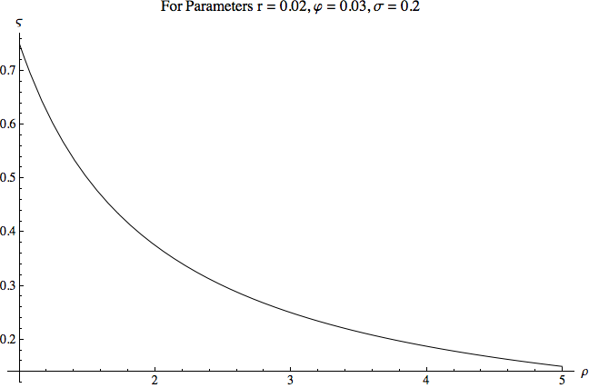
The Approximate Risky Portfolio Share \riskyshare Declines as Relative Risk Aversion \CRRA Increases — Figure 1:The Approximate Risky Portfolio Share $\riskyshare$ Declines as Relative Risk Aversion $\CRRA$ Increases

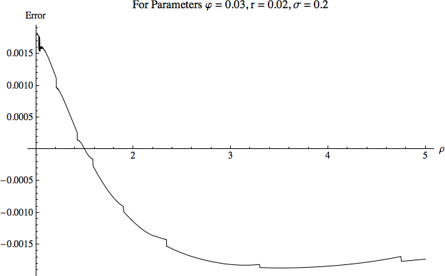
The Approximation Error for the Portfolio Share in Risky Assets \riskyshare Is Small — Figure 2:The Approximation Error for the Portfolio Share in Risky Assets $\riskyshare$ Is Small

Alternative subfigure implementation (commented out in original LaTeX due to HTML rendering issues)

\begin{figure}[h]
\caption{The Risky Portfolio Share $\riskyshare$ and Relative Risk Aversion $\CRRA$} \label{fig:Port}\centering
\subfigure[The Approximate Risky Portfolio Share $\riskyshare$ Declines as Relative Risk Aversion $\CRRA$ Increases]{
    \label{fig:Port:a}
    \fbox{\includegraphics[width=6in]{./Figures/ShareVsCRRA}}
}\\
\vspace{.1in} \subfigure[The Approximation Error for the Portfolio Share in Risky Assets $\riskyshare$ Is Small] {
    \label{fig:Port:b}
    \fbox{\includegraphics[width=6in]{./Figures/ShareApproxErr}}
} \begin{flushleft} \footnotesize Note: The approximation error is computed by solving for the exactly optimal
portfolio share numerically.  See the \texttt{Portfolio-CRRA-Derivations.nb} Mathematica notebook for details.
\end{flushleft}
\end{figure}

1Appendix: The Campbell & Viceira (2002) Approximation¶

For mathematical analysis (especially under the assumption of CRRA utility) it would be convenient if we could approximate the realized arithmetic portfolio return factor by the log of the realized geometric return factor $\Rport_{t+1}=\Rfree^{1-\riskyshare}\Risky_{t+1}^{\riskyshare}$ , because then the logarithm of the return factor would be $\rport_{t+1} = \rfree (1-\riskyshare)+\risky_{t+1}\riskyshare = \rfree + (\risky_{t+1}-\rfree)\riskyshare = \rfree + \EpremLog_{t+1} \riskyshare$ and the realized “portfolio excess return” would be simply $\rport_{t+1}-\rfree = \riskyshare\EpremLog_{t+1}$ . Unfortunately, for $\riskyshare$ values well away from 0 and 1 (that is, for any interesting values of portfolio shares), the log of the geometric mean is a badly biased approximation to the log of the arithmetic mean when the variance of the risky asset is substantial.

Campbell & Viceira (2002) propose instead

\begin{gathered}\begin{aligned} \rport_{t+1} & \approx \rfree+ \riskyshare \EpremLog_{t+1}+\riskyshare \sigma^{2}_{\risky}/2 - \riskyshare^{2}\sigma^{2}_{\risky}/2 \end{aligned}\end{gathered}

(14)

To see one virtue of this approximation,^[11] note (using NormTimes and SumNormsIsNorm) that since the mean and variance of $\EpremLog_{t+1} \riskyshare$ are respectively $\riskyshare(\risky - \sigma^{2}_{\risky}/2- \rfree)$ and $\riskyshare^{2} \sigma^{2}_{\risky}$ , fact LogELogNormTimes implies that

\begin{gathered}\begin{aligned} \log \Ex_{t}[e^{\EpremLog_{t+1} \riskyshare}] & = \riskyshare (\risky - \rfree - \sigma^{2}_{\risky}/2) + \riskyshare^{2}\sigma^{2}_{\risky}/2 \end{aligned}\end{gathered}

(15)

which means that exponentiating then taking the expectation then taking the logarithm of (5) gives

\begin{gathered}\begin{aligned} \log \Ex_{t}[e^{\rport_{t+1}}] & = \log e^{\rfree} + \log \Ex_{t}[e^{\riskyshare \EpremLog_{t+1}}] + \log e^{\riskyshare\sigma^{2}_{\risky}/2 - \riskyshare^{2}\sigma^{2}_{\risky}/2} \\ & = \rfree + \riskyshare (\risky-\rfree-\sigma^{2}_{\risky}/2)+\riskyshare^{2}\sigma^{2}_{\risky}/2 +\riskyshare \sigma^{2}_{\risky}/2 - \riskyshare^{2}\sigma^{2}_{\risky}/2 \\ \log \Ex_{t}[e^{\rport_{t+1}}] - \rfree & = \riskyshare (\risky-\rfree) \end{aligned}\end{gathered}

(16)

or, in words: The expected excess portfolio return is equal to the proportion invested in the risky asset times the expected return of the risky asset.^[12]

Footnotes¶

$\uFunc(\cRat) = (1-\CRRA)^{-1}\cRat^{1-\CRRA}$ .
↩
Both papers present the solution in the case with multiple risky assets; for the two-asset case, see the CRRA Portfolio Choice with Two Risky Assets.
↩
The MathFactsList tells us that a variable with this lognormal distribution has an expected return factor of $\Ex_{t}[e^{\risky_{t+1}}]=e^{\risky}=\Risky$ (where upper-case variables like $\Risky$ without a subscript are the time-invariant mean).
↩
A common interpretation is that this is the problem of a retired investor who expects to receive no further labor income. Note however that all risks other than the returns from financial investments have been ruled out; for example, health expense risk is not possible in this model, though recent research has argued such risk is important (maybe even dominant) later in life (cf. Ameriks et al. (2011)).
↩
Riskless labor income can trivially be added to the problem, because its risklessness means that (in the absence of liquidity constraints) it is indistinguishable from a lump sum of extra current wealth with a value equal to the present discounted value (using the riskless rate) of the (riskless) future labor income. Of course, in practice, labor income is not riskless, but when labor income is risky the problem no longer has the tidy analytical solution described here and must be solved numerically. See Carroll (2023) for an introduction to numerical solution methods.
↩
Samuelson (1979).
↩
Google “arithmetic geometric mean wiki” for a refresher on the difference between arithmetic and geometric means. If the portfolio return is instead geometric $\Rfree^{1-\riskyshare}\Risky^{\riskyshare}$ then the approximate formulas below become exact.
↩
See the appendix for further details.
↩
This expression differs slightly from that derived by Campbell & Viceira (2002), because we adjust the mean logarithmic return of the risky investment for its variance in order to keep the mean return factor constant for different values of the variance (cf. (4)), which makes comparisons of alternative levels of risk more transparent.
↩
See the appendix for a figure showing the quality of the approximation.
↩
The approximation is motivated by the continuous-time solution, which is obtained using Ito’s lemma.
↩
We use the word “return” always to mean the logarithm of the corresponding “factor”; and when not explicitly specified, we always take the expectation before taking the log; if we wanted to refer to $\Ex_{t}[\rport_{t+1}]$ we would call it the expected log portfolio return (to distinguish it from the expected portfolio return, $\log \Ex_{t}[e^{\rport_{t+1}}]$ ).
↩

References¶

Merton, R. C. (1969). Lifetime Portfolio Selection under Uncertainty: The Continuous-Time Case. Review of Economics and Statistics, 51(3), 247–257. 10.2307/1926560
Samuelson, P. A. (1969). Lifetime Portfolio Selection by Dynamic Stochastic Programming. Review of Economics and Statistics, 51, 239–246.
Campbell, J. Y., & Viceira, L. M. (2002). Appendix to Strategic Asset Allocation: Portfolio Choice for Long-Term Investors. Oxford University Press. https://scholar.harvard.edu/files/campbell/files/bookapp.pdf
Mehra, R., & Prescott, E. C. (1985). The Equity Premium: A Puzzle. Journal of Monetary Economics, 15(2), 145–161. 10.1016/0304-3932(85)90061-3
Haliassos, M., & Bertaut, C. C. (1995). Why Do So Few Hold Stocks? The Economic Journal, 105(432), 1110–1129. 10.2307/2235407
Ameriks, J., Caplin, A., Laufer, S., & Van Nieuwerburgh, S. (2011). The Joy Of Giving Or Assisted Living? Using Strategic Surveys To Separate Public Care Aversion From Bequest Motives. The Journal of Finance, 66(2), 519–561.
Carroll, C. D. (2023). Solving Microeconomic Dynamic Stochastic Optimization Problems. Econ-ARK REMARK. https://llorracc.github.io/SolvingMicroDSOPs
Samuelson, P. A. (1979). Why we should not make mean log of wealth big though years to act are long. Journal of Banking and Finance, 3(4), 305–307. http://dx.doi.org/10.1016/0378-4266(79)90023-2