Consider a consumer subject to the dynamic budget constraint
where is beginning-of-period bank balances, is current labor income, and is the constant interest factor. Actual labor income is permanent labor income modified by a transitory shock factor :
where . Permanent labor income grows by a predictable factor from period to period:
PermShks=true:
PermShks=false:
so that the expected present discounted value of permanent labor income (“human wealth”) for an infinite-horizon consumer is
We will assume that the consumer behaves according to the consumption rule
where is the “marginal propensity to consume” out of total wealth .[1]
Under these circumstances, the The Random Walk Model of Consumption shows that consumption will follow a random walk,
Now assume that the economy is populated by a set of measure one of consumers indexed by a superscript distributed uniformly along the unit interval. Per capita values of all variables, designated by the upper case, are the integral over all individuals in the economy, as in the Aggregation For Dummies (Macroeconomists), so that
This equation implies that an aggregate version of equation (7) holds,[2]
In principle, we could allow each individual in this economy to experience a different transitory shock (and, PermShks=true: permanent shock) from every other individual in each period. However, for our purposes it is useful to assume that everyone experiences the same shocks in a given period; that is (PermShks=true: and ).
Assuming (here and henceforth) that the growth factor for permanent income is , the figures below show the path of consumption and bank balances (the solid dots) for an economy populated by omniscient consumers who in periods for had experienced (PermShks=true: ); that is, this economy has had no shocks to income in the past. (For convenience, the consumer is assumed to have arrived in period with ). In period the consumer draws (PermShks=true: and ); thereafter (PermShks=true: ). The figures show and the corresponding values for .
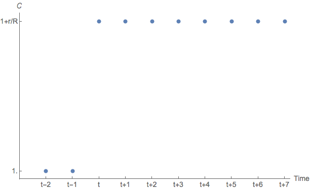
Figure 1:Path of after a shock , Omniscient Consumers
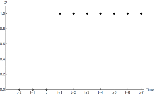
Figure 2:Path of after a shock , Omniscient Consumers
Now suppose that not every consumer updates expectations in every period. Instead, expectations are “sticky”: each consumer updates with probability in each period. Whether the consumer at location updates in period is determined by the realization of the dichotomous random variable
and each period’s updaters are chosen randomly such that a constant proportion update in each period:
It will also be convenient to define the date of consumer ’s most recent update; we call this object . We designate the value of a variable at date for a consumer who last updated his expectations at date by , where the part of the subscript following indicates criteria that must be matched by the consumer’s (or group’s) . To illustrate, consider a consumer who updated his expectations most recently in period so that . This consumer’s actual consumption in period will be , the level of consumption that was chosen in period given beliefs at that time.
We are assuming that the probability of adjusting one’s expectations is independent of the level of income or wealth; therefore, the average levels of wealth and income among those consumers who adjust their expectations this period will be the same as the average levels of wealth and income in the economy as a whole. This independence assumption is crucial for aggregation: it ensures that the subset of consumers who update in any period is representative of the population.
We need a notation to represent sets of consumers defined by the period of their most recent update. We denote such a set by the condition on ; for example, the set of consumers whose most recent update, as of date , was prior to period would be . We denote the per-capita value of a variable , among consumers in a set as of date , by . Dropping the superscripts to reduce clutter, per-capita consumption among households who have updated in period is therefore
Dropping the superscript for notational simplicity, the level of consumption per capita that would prevail if all consumers were to update in period is . But since the set of consumers who updated was randomly selected from the population, the average level of consumption-per-capita for the updaters must equal the average level of consumption-per-capita that would characterize the population as a whole if everyone in the economy were to update. This is the key step that allows aggregation to work analytically.
In periods when expectations are not updated, the consumer continues to spend the same amount as in the most recent period when his expectations were updated.[3] If the economy is large the proportion of consumers who update their expectations every period will be .[4] Average consumption among those who are not updating in the current period (for whom ) is then
because consumption per capita among those who are not updating in the current period is (by assumption) identical to their consumption per capita in the prior period, which must match aggregate consumption per capita in the prior period because the set who do not update today is randomly selected from the population.
Now note that
and
while, defining (PermShks=true: and ),
PermShks=true:
PermShks=false:
where (16) follows its predecessor since, among consumers who have updated in period , the random walk proposition says that . Subtracting from both sides of (16) and substituting the result into (14), and using (15) to substitute for , yields
PermShks=true:
PermShks=false:
where is a white noise variable ().
We are finally in position to show how aggregate consumption and wealth would respond in this economy to a transitory positive shock to aggregate labor income like the one considered above for the omniscient model.
Consider the case of a positive shock of size , as before. In the first period consumption rises only by , rather than the full amount corresponding to the permanent income associated with the new level of wealth. Therefore aggregate wealth in period will be greater than it would have been in the omniscient model. Similarly for all subsequent periods. Thus, in contrast with the omniscient model, the sluggish adjustment of consumption to the shock means that the shock has a permanent effect on the level of aggregate wealth, and therefore on the level of aggregate consumption. (The figures below depict the results.)
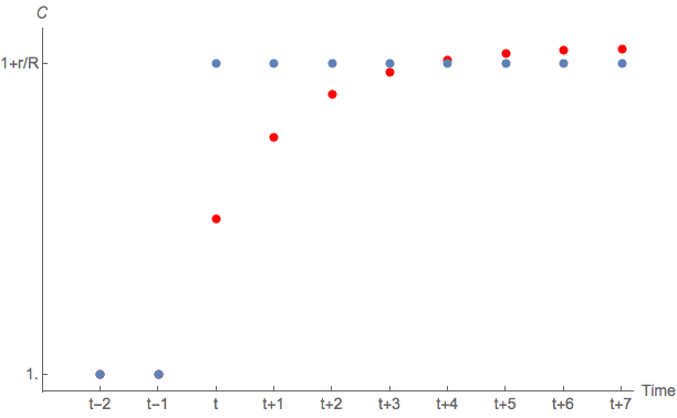
Figure 3:Path of after a shock ; Sticky Expectations in Red/Gray
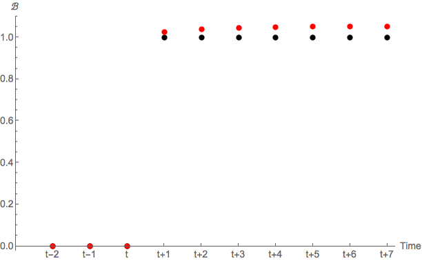
Figure 4:Path of after a shock ; Sticky Expectations in Red/Gray
The sticky expectations model says that consumption growth today can be statistically related to any variable that is related to lagged consumption growth. In particular, if lagged consumption growth is related to lagged income growth (as it certainly will be), then there should be a statistically significant effect of lagged income growth on current consumption growth if expectations are sticky.
If the model derived here could be taken literally, it would suggest estimating an equation of the form
and interpreting the coefficient as a measure of .
However, if there is potential measurement error in the coefficient obtained from estimating (20) would be biased toward zero for standard errors-in-variables reasons (just as regressing consumption on actual income yields a downward-biased estimate of the response of consumption to permanent income), which means that the estimate of would be biased toward 1 (i.e. the omniscient model in which everyone adjusts all the time). Under these circumstances, direct estimation of (20) would not be a reliable way to estimate .
For estimation methods that get around this problem see Sommer (2007), Carroll et al. (2011), Carroll et al. (2011). Those papers consistently find that the proportion of updaters is about per quarter, so that the serial correlation of “true” consumption growth is about per quarter.
1Appendix
This appendix provides additional derivations and notation useful for simulating the model. One way of interpreting consumers’ behavior in this model is to attribute to them the beliefs that would rationalize their actions. Define as the level of wealth (human and nonhuman) that the consumer perceives. Then the Deaton definition of the permanent income hypothesis is that
and the reason consumption follows a random walk is that is precisely the amount that ensures that .
Writing the “believed” level of wealth as , we could then interpret the failure of the sticky expectations consumer to change his consumption during the period of nonupdating as reflecting his optimal forecast that, in the absence of further information, .
To pursue this interpretation, it is useful to write the budget constraint more explicitly, as before; start with the constraint in levels, then decompose variables into ratios to permanent income (nonbold variables) and the level of permanent income:
where we permit a time subscript on and because we want to allow for the possibility that beliefs about the interest rate or growth rate might change over time. (PermShks=false: We also allow henceforth for the existence of permanent shocks to income, .)
Consider an economy that comes into existence in period 0 with a population of consumers who are identical in every respect, including their beliefs about current and future values of the economy’s variables.
First we examine the case where neither nor can change after date 0. In that case, we can track the dynamics of believed and actual variables as follows.
where capturing the dynamics of the ratio of true permanent income to believed permanent income requires us to compute
and so
with the crucially useful fact that since by assumption neither nor is changing, normalized human wealth does not change from
so that
so that perceived wealth and consumption will be
Matters are more complex if expectations about and are allowed to change over time.
Suppose again that we begin our economy in period 0 with population with homogeneous views: Everyone believes and ; so long as these views are universally held in the population, aggregate dynamics are captured by the foregoing analysis.
Suppose, however, that in some period the economy’s “true” values of or change. Updating consumers see this change immediately. But nonupdaters will not discover the changed nature of the economy’s dynamics until they update again.
We capture this modification to the model by keeping track of the aggregate values of the variables for the set of consumers who adhere to each differing opinion, along with the population mass associated with the different opinions. Specifically, suppose there are different opinions in the population, each of whom constitutes population mass such that . Then for each such population, it will be necessary to keep track of their average beliefs about macroeconomic variables.
Suppose, for example, that through period there have been only different opinion groups in the population. In period either or changes. We need then to define group by and and to define , , and so on. We will henceforth need to keep track of dynamics of the consumers who remain in belief group by, e.g.,
while we need to keep track of the populations of the differing groups by, e.g.,
and so on. These population dynamics continue forever, but the population of households continuing to hold any specific belief configuration dwindles toward zero as time progresses.
Aggregate variables for the population as a whole can be constructed as the population-weighted sums across all the differing belief groups, weighted by their masses:
and note that if beliefs change back to a configuration that has been seen before it is possible to add the population mass and aggregate values of the variables associated with the new population with that belief configuration to the corresponding figures for the old population that holds the same beliefs. This reduces the number of groups that the simulations must track in the case where beliefs switch between a limited number of distinct values.
This is the optimal consumption function for a utility-maximizing consumer with if that consumer has quadratic utility (Hall (1978)) or if the consumer has CRRA utility and perfect foresight and anticipates . See the Consumption Functions and the Permanent Income Hypothesis for a derivation of this consumption function under quadratic utility, and Consumption Under Perfect Foresight and CRRA Utility for the derivation in the perfect foresight CRRA case. Deaton (1992) argues that the “Permanent Income Hypothesis” should be defined as the hypothesis that consumption is determined according to (6); but this differs sharply from Friedman (1957)’s definition, and has not become universally accepted.
The crucial feature of the model that allows us to aggregate analytically is the linearity of the consumption rule in and .
This makes sense because under the Hall (1978) assumptions the expected change in consumption is zero under our assumption that .
For consumers who are not updating at date , but , so the integral produces the sum of consumption among only those who are updating in period .
- Sommer, M. (2007). Habit Formation and Aggregate Consumption Dynamics. The B.E. Journal of Macroeconomics, 7(1). 10.2202/1935-1690.1444
- Carroll, C. D., Sommer, M., & Slacalek, J. (2011). International Evidence on Sticky Consumption Growth. Review of Economics and Statistics, 93(4), 1135–1145. 10.1162/REST_a_00122
- Carroll, C. D., Otsuka, M., & Slacalek, J. (2011). How Large Are Housing and Financial Wealth Effects? A New Approach. Journal of Money, Credit and Banking, 43(1), 55–79. 10.1111/j.1538-4616.2010.00365.x
- Hall, R. E. (1978). Stochastic Implications of the Life-Cycle/Permanent Income Hypothesis: Theory and Evidence. Journal of Political Economy, 86(6), 971–987. 10.1086/260724
- Deaton, A. S. (1992). Understanding Consumption. Oxford University Press.
- Friedman, M. A. (1957). A Theory of the Consumption Function. Princeton University Press.