The Brock-Mirman Stochastic Growth Model
Brock & Mirman (1972)
The social planner’s goal is to solve the problem:
max E [ ∑ n = 0 ∞ β n log C t + n ] \max ~~ \Ex\left[ \sum_{n=0}^{\infty} \Discount^{n} \log \Cons_{t+n}\right] max E [ n = 0 ∑ ∞ β n log C t + n ] s.t. K t + 1 = Y t − C t Y t + 1 = A t + 1 K t + 1 α \begin{gathered}\begin{aligned}
& \text{s.t.} \nonumber
\\ \Kap_{t+1} & = \Inc_{t}-\Cons_{t}
\\ \Inc_{t+1} & = \PtyLev_{t+1} \Kap_{t+1}^{\kapShare}
\end{aligned}\end{gathered} K t + 1 Y t + 1 s.t. = Y t − C t = A t + 1 K t + 1 α where A t \PtyLev_{t} A t t t t
that the depreciation rate on capital is 100 percent.
In this model the capital stock is not useful as a state variable: Because capital has a 100 percent depreciation rate, all that matters to the consumer when choosing how much to consume is how much income they have now, and not how that income breaks down into a part due to K \Kap K A \PtyLev A
The first step is to rewrite the problem in Bellman equation form
V t ( Y t ) = max C t log C t + β E t [ V t + 1 ( Y t + 1 ) ] \Value_{t}(\Inc_{t}) = \max_{\Cons_{t}} ~~ \log \Cons_{t} + \Discount \Ex_{t} [\Value_{t+1}(\Inc_{t+1})] V t ( Y t ) = C t max log C t + β E t [ V t + 1 ( Y t + 1 )] and take the first order condition:
u ′ ( C t ) = β E t [ A t + 1 α K t + 1 α − 1 u ′ ( C t + 1 ) ] 1 C t = β E t [ A t + 1 α K t + 1 α − 1 C t + 1 ] 1 = β E t [ α A t + 1 K t + 1 α − 1 ⏟ ≡ R t + 1 C t C t + 1 ] \begin{gathered}\begin{aligned}
\uP(\Cons_{t}) & = \Discount \Ex_{t}\left[\PtyLev_{t+1} \kapShare \Kap_{t+1}^{\kapShare-1} \uP(\Cons_{t+1})\right] \\
\frac{1}{\Cons_{t}} & = \Discount \Ex_{t}\left[\frac{\PtyLev_{t+1} \kapShare \Kap_{t+1}^{\kapShare-1}}{\Cons_{t+1}}\right] \\
1 & = \Discount \Ex_{t} \left[\underbrace{\kapShare \PtyLev_{t+1} \Kap_{t+1}^{\kapShare-1}}_{\equiv \Risky_{t+1}}\frac{\Cons_{t}}{\Cons_{t+1}}\right]
\end{aligned}\end{gathered} u ′ ( C t ) C t 1 1 = β E t [ A t + 1 α K t + 1 α − 1 u ′ ( C t + 1 ) ] = β E t [ C t + 1 A t + 1 α K t + 1 α − 1 ] = β E t ⎣ ⎡ ≡ R t + 1 α A t + 1 K t + 1 α − 1 C t + 1 C t ⎦ ⎤ where our definition of R t + 1 \Risky_{t+1} R t + 1
to the usual consumption Euler equation (and you should think about why this is the
right definition of the interest factor in this model).
Now we show that this FOC is satisfied by the consumption function C t = κ Y t \Cons_{t} = \MPC \Inc_{t} C t = κ Y t κ = 1 − α β \MPC = 1-\kapShare \Discount κ = 1 − α β
first that the proposed consumption rule implies that K t + 1 = ( 1 − κ ) Y t \Kap_{t+1} = (1-\MPC) \Inc_{t} K t + 1 = ( 1 − κ ) Y t
The first order condition says
1 = β E t [ α A t + 1 K t + 1 α K t + 1 κ Y t κ Y t + 1 ] = β E t [ α Y t + 1 K t + 1 κ Y t κ Y t + 1 ] = β E t [ α Y t K t + 1 ] = β E t [ α Y t Y t − C t ] = β E t [ α Y t Y t ( 1 − κ ) ] = β E t [ α 1 ( 1 − κ ) ] ( 1 − κ ) = α β κ = 1 − α β . \begin{gathered}\begin{aligned}
1 & = \Discount \Ex_{t} \left[\kapShare \frac{\PtyLev_{t+1} \Kap_{t+1}^{\kapShare}}{\Kap_{t+1}}\frac{\MPC \Inc_{t}}{\MPC \Inc_{t+1}}\right]
\\ & = \Discount \Ex_{t} \left[\kapShare \frac{\Inc_{t+1}}{\Kap_{t+1}}\frac{\MPC \Inc_{t}}{\MPC \Inc_{t+1}}\right]
\\ & = \Discount \phantom{\Ex_{t}} \left[\kapShare \frac{\Inc_{t}}{\Kap_{t+1}}\right]
\\ & = \Discount \phantom{\Ex_{t}} \left[\kapShare \frac{\Inc_{t}}{\Inc_{t}-\Cons_{t}}\right]
\\ & = \Discount \phantom{\Ex_{t}} \left[\kapShare \frac{\Inc_{t}}{\Inc_{t}(1-\MPC)}\right]
\\ & = \Discount \phantom{\Ex_{t}} \left[\kapShare \frac{1}{(1-\MPC)}\right]
\\ (1-\MPC) & = \kapShare \Discount
\\ \MPC & = 1-\kapShare \Discount.
\end{aligned}\end{gathered} 1 ( 1 − κ ) κ = β E t [ α K t + 1 A t + 1 K t + 1 α κ Y t + 1 κ Y t ] = β E t [ α K t + 1 Y t + 1 κ Y t + 1 κ Y t ] = β E t [ α K t + 1 Y t ] = β E t [ α Y t − C t Y t ] = β E t [ α Y t ( 1 − κ ) Y t ] = β E t [ α ( 1 − κ ) 1 ] = α β = 1 − α β . An important way of judging a macroeconomic
model and deciding whether it makes sense is to examine the model’s
implications for the dynamics of aggregate variables. Defining lower
case variables as the log of the corresponding upper case variable,
this model says that the dynamics of the capital stock are given by
K t + 1 = ( 1 − κ ) Y t = α β A t K t α k t + 1 = log α β + a t + α k t \begin{gathered}\begin{aligned}
\Kap_{t+1} & = (1-\MPC) \Inc_{t}
\\ & = \kapShare\Discount \PtyLev_{t}\Kap_{t}^{\kapShare}
\\ \kap_{t+1} & = \log \kapShare\Discount + \ptyLev_{t} + \kapShare \kap_{t}
\end{aligned}\end{gathered} K t + 1 k t + 1 = ( 1 − κ ) Y t = α β A t K t α = log α β + a t + α k t which tells us that the dynamics of the (log) capital stock have two
components: One component (a t \ptyLev_{t} a t
to the aggregate production technology; the other
is serially correlated with coefficient α \kapShare α
to capital’s share in output.
Similarly, since log output is simply y = a + α k \inc = \ptyLev + \kapShare \kap y = a + α k
of output can be obtained from
y t + 1 = a t + 1 + α k t + 1 = α ( log K t + 1 ) + a t + 1 = α ( log α β Y t ) + a t + 1 = α ( y t + log α β ) + a t + 1 \begin{gathered}\begin{aligned}
\inc_{t+1} & = \ptyLev_{t+1} + \kapShare \kap_{t+1}
\\ & = \kapShare (\log \Kap_{t+1}) + \ptyLev_{t+1}
\\ & = \kapShare (\log \kapShare \Discount \Inc_{t}) + \ptyLev_{t+1}
\\ & = \kapShare (\inc_{t} + \log \kapShare \Discount ) + \ptyLev_{t+1}
\end{aligned}\end{gathered} y t + 1 = a t + 1 + α k t + 1 = α ( log K t + 1 ) + a t + 1 = α ( log α β Y t ) + a t + 1 = α ( y t + log α β ) + a t + 1 so the dynamics of aggregate output, like aggregate capital,
reflect a component that mirrors a \ptyLev a
component with serial correlation coefficient α \kapShare α
The simplest assumption to make about the level of technology
is that its log follows a random walk:
a t + 1 = a t + ϵ t + 1 . \begin{gathered}\begin{aligned}
\ptyLev_{t+1} & = \ptyLev_{t} + \epsilon_{t+1}.
\end{aligned}\end{gathered} a t + 1 = a t + ϵ t + 1 . Under this assumption, consider the dynamic effects on the level of
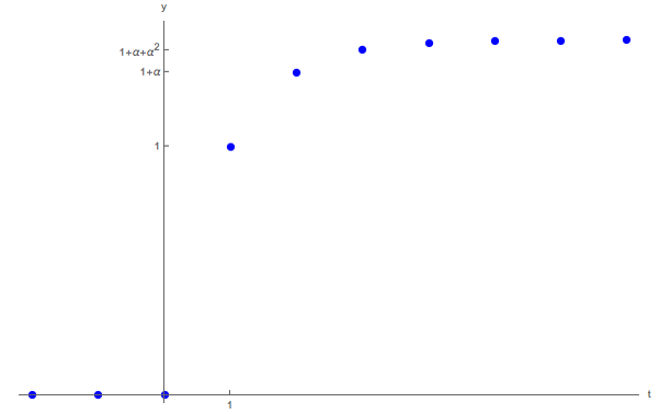
output from a unit positive shock to
the log of technology in period t t t ϵ t + 1 = 1 \epsilon_{t+1}=1 ϵ t + 1 = 1 ϵ s = 0 ∀ s ≠ t + 1 \epsilon_{s} = 0~\forall~s \neq t+1 ϵ s = 0 ∀ s = t + 1
the economy had been at its original steady-state level of output y ˇ \Target{y} y ˇ
in the prior period. Then the expected dynamics of output would be given
by
y t = y ˇ + a t E t [ y t + 1 ] = y ˇ + a t + α a t E t [ y t + 2 ] = y ˇ + a t + α a t + α 2 a t \begin{gathered}\begin{aligned}
\inc_{t} & = \Target{y} + \ptyLev_{t}
\\ \Ex_{t}[\inc_{t+1}] & = \Target{y}+\ptyLev_{t}+\kapShare \ptyLev_{t}
\\ \Ex_{t}[\inc_{t+2}] & = \Target{y}+\ptyLev_{t}+\kapShare \ptyLev_{t}+\kapShare^{2} \ptyLev_{t}
\end{aligned}\end{gathered} y t E t [ y t + 1 ] E t [ y t + 2 ] = y ˇ + a t = y ˇ + a t + α a t = y ˇ + a t + α a t + α 2 a t and so on, as depicted in Figure 1
Figure 1: Dynamics of Output With a Random Walk Shock
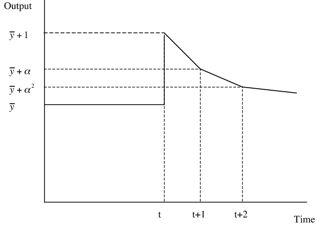
Also interesting is the case where the level of
technology follows a white noise process,
a t + 1 = a ˇ + ϵ t + 1 . \begin{gathered}\begin{aligned}
\ptyLev_{t+1} & = \Target{\ptyLev} + \epsilon_{t+1}.
\end{aligned}\end{gathered} a t + 1 = a ˇ + ϵ t + 1 . The dynamics of income in this case are depicted in Figure 2
Figure 2: Dynamics of Output With A White Noise Shock
The key point of this analysis, again, is that the dynamics of the model
are governed by two components: The dynamics of the technology shock, and
the assumption about the saving/accumulation process.
For further analysis, consider a nonstochastic version of this model,
with A t = 1 ∀ t \PtyLev_{t} = 1 ~ \forall ~ t A t = 1 ∀ t
C t + 1 C t = ( β R t + 1 ) 1 / ρ \begin{gathered}\begin{aligned}
\frac{\Cons_{t+1}}{\Cons_{t}} & = (\Discount \Rfree_{t+1})^{1/\CRRA} \\
\end{aligned}\end{gathered} C t C t + 1 = ( β R t + 1 ) 1/ ρ But this is an economy with no technological progress, so the steady-state
interest rate must take on the value such that C t + 1 / C t = 1 \Cons_{t+1}/\Cons_{t}=1 C t + 1 / C t = 1
must have β R = 1 \Discount \Rfree = 1 β R = 1 R = 1 / β \Rfree = 1/\Discount R = 1/ β
We can further derive the steady state level of capital of a nonstochastic version of the model in which a t = a ∀ t \ptyLev_{t}=\ptyLev~\forall~t a t = a ∀ t
from (6)
k = log α β + a + α k ( 1 − α ) k = log α β + a k = log α β + a 1 − α \begin{gathered}\begin{aligned}
\kap & = \log \kapShare\Discount + \ptyLev + \kapShare \kap
\\ (1-\kapShare) \kap & = \log \kapShare\Discount + \ptyLev
\\ \kap & = \frac{\log \kapShare\Discount + \ptyLev}{1-\kapShare}
\end{aligned}\end{gathered} k ( 1 − α ) k k = log α β + a + α k = log α β + a = 1 − α log α β + a The nonstochastic version of the model is of course not very interesting, except as a point of comparison to the stochastic version of the model. But what could be meant by the ‘steady state’ of a stochastic mdoel that never settles down? We can define a ‘stochastic steady state’ for such models in a number of (potentially) different ways:
The location (if one exists) to which the model will converge after an arbitrarily long period in which no shocks occurred a t + 1 = a t ∀ t \ptyLev_{t+1}=\ptyLev_{t}~\forall~t a t + 1 = a t ∀ t expect that shocks will occur)
The mean value of some variable in the model (say, K \Kap K
The value of some state variable, say K ˇ \Target{\Kap} K ˇ E t [ K t + 1 ] = K t \Ex_{t}[\Kap_{t+1}] = \Kap_{t} E t [ K t + 1 ] = K t K t = K ˇ \Kap_{t}=\Target{\Kap} K t = K ˇ
We consider here the last of these, which we will show reduces (in this special case) to the same equation as for the nonstochastic version of the model, K t + 1 = K t \Kap_{t+1}=\Kap_{t} K t + 1 = K t
1 = β E t [ α A t + 1 K t + 1 α − 1 ⏟ ≡ R t + 1 C t C t + 1 ] 1 = β E t [ α A t + 1 K t + 1 α − 1 Y t Y t + 1 ] 1 = β E t [ α A t + 1 K t + 1 α − 1 A t K t α A t + 1 K t + 1 α ] 1 = β E t [ α K t + 1 α − 1 A t K t α K t + 1 α ] 1 = β [ α K t + 1 α − 1 A t K t α K t + 1 α ] \begin{gathered}\begin{aligned}
1 & = \Discount \Ex_{t} \left[\underbrace{\kapShare \PtyLev_{t+1} \Kap_{t+1}^{\kapShare-1}}_{\equiv \Risky_{t+1}}\frac{\Cons_{t}}{\Cons_{t+1}}\right]
\\ 1 & = \Discount \Ex_{t} \left[\kapShare \PtyLev_{t+1} \Kap_{t+1}^{\kapShare-1}\frac{Y_{t}}{Y_{t+1}}\right]
\\ 1 & = \Discount \Ex_{t} \left[\kapShare \PtyLev_{t+1} \Kap_{t+1}^{\kapShare-1}\frac{\PtyLev_{t} \Kap_{t}^{\kapShare}}{\PtyLev_{t+1} \Kap_{t+1}^{\kapShare}}\right]
\\ 1 & = \Discount \Ex_{t} \left[\kapShare \Kap_{t+1}^{\kapShare-1}\frac{\PtyLev_{t} \Kap_{t}^{\kapShare}}{\Kap_{t+1}^{\kapShare}}\right]
\\ 1 & = \Discount \left[\kapShare \Kap_{t+1}^{\kapShare-1}\frac{\PtyLev_{t} \Kap_{t}^{\kapShare}}{\Kap_{t+1}^{\kapShare}}\right]
% \\ 1 & = \Discount \left[\kapShare \frac{\PtyLev_{t} \Kap_{t}^{\kapShare}}{\Kap_{t+1}}\right]
\end{aligned}\end{gathered} 1 1 1 1 1 = β E t ⎣ ⎡ ≡ R t + 1 α A t + 1 K t + 1 α − 1 C t + 1 C t ⎦ ⎤ = β E t [ α A t + 1 K t + 1 α − 1 Y t + 1 Y t ] = β E t [ α A t + 1 K t + 1 α − 1 A t + 1 K t + 1 α A t K t α ] = β E t [ α K t + 1 α − 1 K t + 1 α A t K t α ] = β [ α K t + 1 α − 1 K t + 1 α A t K t α ] where the expectations operator disappears because no variables are stochastic (the A t + 1 ′ s \PtyLev_{t+1}'s A t + 1 ′ s K t + 1 \Kap_{t+1} K t + 1 t t t A t \PtyLev_{t} A t K t + 1 = K t = K ˇ \Kap_{t+1}=\Kap_{t}=\Target{\Kap} K t + 1 = K t = K ˇ
1 = β α A t K ˇ t α − 1 k ˇ = log β α + a t 1 − α \begin{gathered}\begin{aligned}
1 & = \Discount \kapShare \PtyLev_{t} \Target{\Kap}_{t}^{\kapShare-1}
\\ \Target{\kap} & = \frac{\log \Discount \kapShare + \ptyLev_{t}}{1-\kapShare}
\end{aligned}\end{gathered} 1 k ˇ = β α A t K ˇ t α − 1 = 1 − α log β α + a t which is the generalization of the nonstochastic solution derived in (12)
The result that the nonstochastic and stochastic steady states are the same is special to the Brock-Mirman model; it is NOT true of many other models of growth; it occurs here because the linearity of the consumption function, among other special assumptions. Furthermore, the third of our possible definitions of a steady state will generally differ at least a little bit from either of the first two.
Brock, W. A., & Mirman, L. J. (1972). Optimal Economic Growth and Uncertainty: The Discounted Case. Journal of Economic Theory , 4 (3), 479–513. 10.1016/0022-0531(72)90135-4