Ramsey Ramsey (1928), followed much later by Cass Cass (1965) and Koopmans Koopmans (1965), formulated the canonical model of optimal growth for an economy with exogenous ‘labor-augmenting’ technological progress.
1The Budget Constraint
The economy has a perfectly competitive production sector that uses a Cobb-Douglas aggregate production function
to produce output using capital and labor.[1]
and is an index of labor productivity that grows at rate
Thus, technological progress allows each worker to
produce perpetually more as time goes by with the same amount of
physical capital.[2]
units’ of labor in the economy.
Aggregate capital accumulates according to
Lower case variables are the upper case version divided by efficiency units, i.e.
Note that
which means that (4) can be divided by and becomes
A steady-state will be a point where .
Equation (7) yields a first candidate for an optimal
steady-state of the growth model: It seems reasonable to argue that the best
possible steady-state is the one that maximizes . This is the
“golden rule” optimality condition of
Phelps Phelps (1961), an article well worth reading; this is
one of the chief contributions for which Phelps won the Nobel prize.
2The Social Planner’s Problem
Now suppose that there is a social planner whose goal is to maximize the discounted
sum of CRRA utility from per-capita consumption:
But . Recall that for a variable growing at rate ,
so if the economy started off in period 0 with productivity , by date we can rewrite
Using (10) and the other results above, we can rewrite the social planner’s objective function as
Thus, defining and normalizing the initial
level of productivity to , the complete optimization problem
can be formulated as
subject to
which has a discounted Hamiltonian representation
The first discounted Hamiltonian optimization condition requires {math}\partial \Ham/\partial \cons = 0:
The second discounted Hamiltonian optimization condition requires:
where the definition of is motivated by thinking of
as the interest rate net of depreciation and
dilution.
This is called the “modified golden rule” (or sometimes the
“Keynes-Ramsey rule” because it was originally derived by
Ramsey with an explanation attributed to Keynes).
Thus, we end up with an Euler equation for consumption growth that is
just like the Euler equation in the perfect foresight partial equilibrium consumption model, except that now the relevant interest rate can vary over
time as varies.
Substituting in the modified time preference rate gives
and finally note that defining per capita consumption
so that ,
and since (17) can be written
we have
so the formula for per capita consumption growth (as a function of
) is identical to the model with no growth (equation
(17) with ). Any important differences between
the no-growth model and the model with growth therefore must come
through the channel of differences in .
3The Steady State
The assumption of labor augmenting technological progress was made
because it implies that in steady-state, per-capita consumption, income,
and capital all grow at rate .[3]
implies that at the steady-state value of ,
Thus, the steady-state will be higher if capital
is more productive ( is higher), and will be lower if
consumers are more impatient, population growth is faster,
depreciation is greater, or technological progress occurs more rapidly.
4A Phase Diagram
While the RCK model has an analytical solution for its steady-state,
it does not have an analytical solution for the transition to the
steady-state. The usual method for analyzing
models of this kind is a phase diagram in and .
The first step in constructing the phase diagram is to take the differential
equations that describe the system and find the points where they are
zero. Thus, from (7) we have that implies
and we have already solved for the (constant) that characterizes
the locus. These can be combined to generate the borders between the phases in the phase diagram, as illustrated in Figure 1.
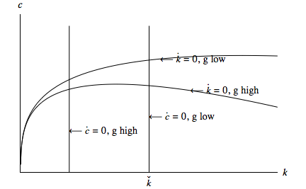
Figure 1: and Loci
5Transition
Actually, as stated so far, the solution to the problem is very simple: The
consumer should spend an infinite amount in every period. This solution is
not ruled out by anything we have yet assumed (except possibly the fact that
once becomes negative the production function is undefined).
Obviously, this is not the solution we are looking for. What is missing is
that we have not imposed anything corresponding to the intertemporal
budget constraint. In this context, the IBC takes the form of a “transversality
condition,”
The intuitive purpose of this unintuitive equation is basically to prevent
the capital stock from becoming negative or infinity as time goes by.
Obviously a capital stock that was negative for the entire future could not
satisfy the equation. And a capital stock that is too large will have
an arbitrarily small interest rate, which will result in the LHS of the
TVC being a positive number, again failing to satisfy the TVC.
Figure 2 shows three paths for and
that satisfy (17) and (7). The topmost path,
however, is clearly on a trajectory toward zero then negative
, while the bottommost path is heading toward an infinite
. Only the middle path, labelled the “saddle path,” satisfies
both (17) and (7) as well as the TVC
(23).
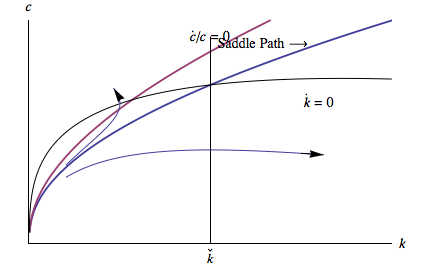
Figure 2:Transition to the Steady State
6Interactive Notebooks
An explicit numerical solution to the Ramsey problem, with a description of a solution method and its
mathematical/computational underpinnings, is available here.
7Appendix: Numerical Solution
The RCK model does not have an analytical solution, which means that
numerical methods must be used to find out the model’s quantitative
implications for transition paths.
The method of solution of these kinds of models is not important for
the purposes of first year graduate macroeconomics; this appendix
has been written as a reference for more advanced students who might
be beginning their research on growth models.
The most straightforward method of numerical solution for perfect foresight
models of this kind is called the
‘time elimination’ method. It starts from the fact that
Note from (17) that we can write
so we can obtain
which is a differential equation with no analytical solution. Many numerical math packages can solve differential equations numerically, yielding a numerical version of the function.
There is one problem, however, which is that at the steady-state values of and both numerator and denominator of this equation are zero. The alternative is to solve the differential equation twice: Once for a domain extending from to , yielding , and once for a domain from to some large value of , yielding . The true consumption policy function can then be approximated by interpolating between the upper endpoint of and the lower endpoint of .
For further details of the numerical solution of this model, see this Jupyter notebook, or clone the repo and, in the cloned directory, run the corresponding python program: ipython RamseyCassKoopmans.py.
The ancient Greek philosophers captured eternal truths; therefore, Greek letters represent constants whose value never changes.
This is the definition of ‘labor-augmenting’ (Harrod-neutral) productivity growth; with a Cobb-Douglas production function, it turns out to be essentially the same as ‘capital-augmenting’ productivity growth, also known as Hicks-neutral, as well as output-neutral (‘Solow-neutral’) progress. The quantity is known as the number of ‘efficiency
See Grossman et al. (2016) for a discussion of the realism of this requirement.
- Ramsey, F. P. (1928). A Mathematical Theory of Saving. Economic Journal, 38(152), 543–559. 10.2307/2224098
- Cass, D. (1965). Optimum Growth in an Aggregative Model of Capital Accumulation. Review of Economic Studies, 32, 233–240. 10.2307/2295827
- Koopmans, T. C. (1965). On the concept of optimal economic growth. In (Study Week on the) Econometric Approach to Development Planning (pp. 225–287). North-Holland Publishing Co., Amsterdam.
- Phelps, E. S. (1961). The Golden Rule of Accumulation. American Economic Review, 638–642.
- Grossman, G. M., Helpman, E., Oberfield, E., & Sampson, T. (2016). Balanced Growth Despite Uzawa (Working Paper No. 21861; Working Paper Series). National Bureau of Economic Research. 10.3386/w21861