Economic agents face risks of many kinds, which may mutually
covary. A stock broker, for example, is likely to earn a salary
bonus that is positively related to the performance of the stock
market; if that broker also has personal stock investments, his
financial wealth and labor income will be positively correlated.
The first part of this section presents a convenient (and empirically
realistic) formulation in which a consumer faces two shocks (which can
be interpreted as a shock to noncapital income and a shock to the rate
of return) that are distributed according to a multivariate lognormal
that allows for correlation between them. The second part describes a
computationally simple and convenient method for approximating that joint
distribution.
1Theory
Consider a consumer who faces both a risk to transitory noncapital income[1]
and a risky log rate-of-return that is affected by following factors: the riskless rate ;
a risk premium ; an additional constant (whose purpose will become clear below); a component
that is linearly related to ; and an independent shock {math}\ShkMeanOneLog_{2} \sim \mathcal{N}(-0.5 \sigma^{2}_{2},\sigma^{2}_{2}):
for some constant . Since is the only component of that covaries with ,
Equation (2) yields a description of the return process
in which the parameter controls the correlation between the
risky log return shock and the risky log labor income shock. If
the processes are independent.
Now we want to find the value of such that the mean risky
return is unaffected by (so that we will be able to
understand clearly the distinct effects of labor income risk, the
independent component of rate-of-return risk , and the
correlation between labor income risk and rate-of-return risk,
). Thus, we want to find the such that
regardless of the values of and . We therefore need:
Using standard facts about lognormals (cf. ), and for convenience
defining , we have
Alternative representation (commented out)
2Computation
A key step in the computational solution of any model with uncertainty is the calculation
of expectations. Writing and and , the expectation of some function that depends on the realization of
the risky return and the labor income shock is:
where is the joint cumulative distribution
function. Standard numerical computation software can compute this
double integral, but at such a slow speed as to be almost unusable.
Computation of the expectation can be massively speeded up by
advance construction of a numerical approximation to
.
Such approximations generally take the approach of replacing the distribution function
with a discretized approximation to it; appropriate weights are attached to
each of a finite set of points indexed by and , and
the approximation to the integral is given by:
where the and matrices contain the conditional means of the two variables in each of the regions. Various methods are used for constructing the weights and the nodes (the and points for
and ).
Perhaps the most popular such method is Gauss-Hermite interpolation (see
Judd (1998) for an exposition, or Kopecky & Suen (2010) for
some alternatives). Here, we will pursue a particularly intuitive
alternative: Equiprobable discretization. In this method, and
boundaries on the joint CDF are determined in such a way as to divide
up the total probability mass into submasses of equal size (each of
which therefore has a mass of ). This is conceptually easier
if we represent the underlying shocks as statistically
independent, as with and above; in that case, each submass is a square region
in the and grid. We then compute the average
value of and conditional on their being
located in each of the subdivisions of the range of the CDF. Since,
in this specification, is a function of , the
values are indexed by both and , but since we have
written as IID, the representation of the approximating
summation is even simpler than (9):
where the function is implicitly defined by (2).
Details can be found in the Mathematica notebook associated with this
section. A particular example, in which and ,
is illustrated in Figure 1; the red dots reflect the height of the approximation
to the CDF above the conditional mean values for and within each of the equiprobable
regions.
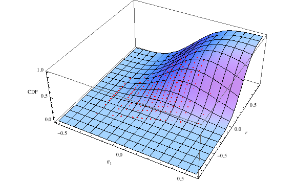
Figure 1:‘True’ CDF With Approximation Points in Red for
The assumed distribution has the property , cf. .
An alternative would be to work with and directly, which would require a multivariate normal with nonzero off-diagonal elements (covariances). The two approaches are mathematically indistinguishable, but the IID representation has certain conveniences for our purposes.
- Judd, K. L. (1998). Numerical Methods in Economics. The MIT Press.
- Kopecky, K. A., & Suen, R. M. H. (2010). Finite State Markov-Chain Approximations To Highly Persistent Processes. Review of Economic Dynamics, 13(3), 701–714. 10.1016/j.red.2010.02.002