Equiprobable Approximation to Bivariate Lognormal Returns
This section starts by defining a convenient notation to represent two rate-of-return shocks
that are distributed according to a multivariate lognormal that allows
for nonzero covariances. It next presents a computationally
simple method for constructing a numerical approximation to that joint distribution. The final
section uses both the numerical approximation, and more accurate (but enormously slower) standard numerical integration tools to assess the accuracy of the Campbell-Vicera analytical approximation to the solution to the optimal portfolio choice problem
described in Portfolio-Multi-CRRA .
1 Statistical Theory ¶ Consider a set of two normally distributed risks
θ 2 , t + 1 ∼ N ( − 0.5 Σ 2 , Σ 2 ) θ 1 , t + 1 ∼ N ( − 0.5 ( x Σ ) 2 , ( x Σ ) 2 ) \begin{gathered}\begin{aligned}
\ShkMeanOneLog_{2,t+1} & \sim \mathcal{N}(-0.5 \sigAll^{2},\sigAll^{2})
\\ \ShkMeanOneLog_{1,t+1} & \sim \mathcal{N}(-0.5 (\scale \sigAll)^{2},(\scale \sigAll)^{2})
\end{aligned}\end{gathered} θ 2 , t + 1 θ 1 , t + 1 ∼ N ( − 0.5 Σ 2 , Σ 2 ) ∼ N ( − 0.5 ( x Σ ) 2 , ( x Σ ) 2 ) which are statistically independent (θ 1 , t + 1 ⊥ θ 2 , t + 1 \ShkMeanOneLog_{1,t+1} \perp \ShkMeanOneLog_{2,t+1} θ 1 , t + 1 ⊥ θ 2 , t + 1
standard deviation is determined by the proportionality factor
x \scale x
Σ \sigAll Σ
by changing Σ \sigAll Σ x \scale x
The θ \ShkMeanOneLog θ Θ \ShkMeanOne Θ
of the levels are independent of the size of the risk (cf. ). That is, defining Θ i = E t [ e θ i , t + 1 ] \ShkMeanOne_{i} = \Ex_{t}[e^{\ShkMeanOneLog_{i,t+1}}] Θ i = E t [ e θ i , t + 1 ] i ∈ { 1 , 2 } i \in \{1,2\} i ∈ { 1 , 2 }
Θ i ≡ E t [ Θ i , t + 1 ] = 1 ∀ i log E t [ Θ i , t + 1 ] = 0 ∀ i . \begin{gathered}\begin{aligned}
\ShkMeanOne_{i} \equiv \Ex_{t}[\ShkMeanOne_{i,t+1}] & = 1~\forall~i
\\ \log \Ex_{t}[\ShkMeanOne_{i,t+1}] & = 0~\forall~i.
\end{aligned}\end{gathered} Θ i ≡ E t [ Θ i , t + 1 ] log E t [ Θ i , t + 1 ] = 1 ∀ i = 0 ∀ i . From the first shock we can construct a log rate-of-return variable that can be represented equivalently in either of two ways:
( r ˊ 1 , t + 1 = ) ( ) r 1 , t + 1 = r 1 + 0.5 ( x Σ ) 2 ⏞ ≡ r ˊ 1 + θ 1 , t + 1 = r ˊ 1 − 0.5 ( x Σ ) 2 ⏟ = r 1 + 0.5 ( x Σ ) 2 + θ 1 , t + 1 ⏟ ≡ θ 1 , t + 1 \begin{gathered}\begin{aligned}
({\riskyAlt_{1,t+1} = }) ({}) \risky_{1,t+1} & = \overbrace{\risky_{1}+0.5(\scale \sigAll)^{2}}^{\equiv \riskyAlt_{1}}+\ShkMeanOneLog_{1,t+1}
\\ & = \underbrace{\riskyAlt_{1}-0.5(\scale \sigAll)^{2}}_{=\risky_{1}}+\underbrace{0.5(\scale \sigAll)^{2}+\ShkMeanOneLog_{1,t+1}}_{\equiv \ShkLogZeroLog_{1,t+1}}
\end{aligned}\end{gathered} ( r ˊ 1 , t + 1 = ) ( ) r 1 , t + 1 = r 1 + 0.5 ( x Σ ) 2 ≡ r ˊ 1 + θ 1 , t + 1 = = r 1 r ˊ 1 − 0.5 ( x Σ ) 2 + ≡ θ 1 , t + 1 0.5 ( x Σ ) 2 + θ 1 , t + 1 where θ 1 , t + 1 ∼ N ( 0. , ( x Σ ) 2 ) \ShkLogZeroLog_{1,t+1}~\sim~\mathcal{N}(0.,(\scale \sigAll)^{2}) θ 1 , t + 1 ∼ N ( 0. , ( x Σ ) 2 ) θ \ShkLogZeroLog θ θ \ShkMeanOneLog θ
R 1 , t + 1 ( = R ˊ 1 , t + 1 ) ( ) ≡ ( e r ˊ 1 , t + 1 = ) ( ) e r 1 , t + 1 R 1 ( = R ˊ 1 ≡ E t [ R ˊ 1 , t + 1 ] ) ( ) ≡ E t [ R 1 , t + 1 ] = ( e r ˊ 1 + ( x Σ ) 2 / 2 − ( x Σ ) 2 / 2 = e r ˊ 1 = ) ( ) e r 1 + ( x Σ ) 2 / 2 log E t [ R 1 , t + 1 ] ( = log E t [ R ˊ 1 , t + 1 ] ) ( ) = r 1 + ( x Σ ) 2 / 2 = r ˊ 1 \begin{gathered}\begin{aligned}
\Risky_{1,t+1} ({= \acute{\Risky}_{1,t+1}}) ({}) & \equiv ({e^{\riskyAlt_{1,t+1}} =}) ({}) e^{\risky_{1,t+1}}
\\ \Risky_{1} ({= \acute{\Risky}_{1} \equiv \Ex_{t}[\acute{\Risky}_{1,t+1}]}) ({}) \equiv\Ex_{t}[\Risky_{1,t+1}] & = ({e^{\riskyAlt_{1}+(\scale \sigAll)^{2}/2-(\scale \sigAll)^{2}/2}= e^{\riskyAlt_{1}} =}) ({})e^{\risky_{1}+(\scale \sigAll)^{2}/2}
\\ \log \Ex_{t}[\Risky_{1,t+1}] ({= \log \Ex_{t}[\acute{\Risky}_{1,t+1}]}) ({}) & = \risky_{1}+(\scale \sigAll)^{2}/2 = \riskyAlt_{1}
\end{aligned}\end{gathered} R 1 , t + 1 ( = R ˊ 1 , t + 1 ) ( ) R 1 ( = R ˊ 1 ≡ E t [ R ˊ 1 , t + 1 ] ) ( ) ≡ E t [ R 1 , t + 1 ] log E t [ R 1 , t + 1 ] ( = log E t [ R ˊ 1 , t + 1 ] ) ( ) ≡ ( e r ˊ 1 , t + 1 = ) ( ) e r 1 , t + 1 = ( e r ˊ 1 + ( x Σ ) 2 /2 − ( x Σ ) 2 /2 = e r ˊ 1 = ) ( ) e r 1 + ( x Σ ) 2 /2 = r 1 + ( x Σ ) 2 /2 = r ˊ 1 where note to avoid confusion that r ˊ 1 ( = log E t [ R ˊ 1 , t + 1 ] ) ( ) ≠ E t [ ( ) ˊ ( ) r 1 , t + 1 ] \riskyAlt_{1} ({= \log \Ex_{t}[\acute{\Risky}_{1,t+1}]}) ({}) \neq \Ex_{t}[(\acute) (){{\risky}}_{1,t+1}] r ˊ 1 ( = log E t [ R ˊ 1 , t + 1 ] ) ( ) = E t [( ) ˊ ( ) r 1 , t + 1 ]
while log E t [ R 1 , t + 1 ] ≠ r 1 = E t [ r 1 , t + 1 ] \log \Ex_{t}[\Risky_{1,t+1}] \neq \risky_{1}=\Ex_{t}[\risky_{1,t+1}] log E t [ R 1 , t + 1 ] = r 1 = E t [ r 1 , t + 1 ]
Using E t [ θ 2 , t + 1 ] = − 0.5 Σ 2 \Ex_{t}[\ShkMeanOneLog_{2,t+1}] = -0.5 \sigAll^{2} E t [ θ 2 , t + 1 ] = − 0.5 Σ 2 E t [ ( ω / x ) θ 1 , t + 1 ] = − 0.5 ( ( ω / x ) Σ ) 2 \Ex_{t}[(\omega/\scale)\ShkMeanOneLog_{1,t+1}] = -0.5 ((\omega/\scale)\sigAll)^{2} E t [( ω / x ) θ 1 , t + 1 ] = − 0.5 (( ω / x ) Σ ) 2
r 2 , t + 1 ( = r ˊ 2 , t + 1 ) ( ) ≡ r ˊ 2 + ζ + ( ω / x ) θ 1 , t + 1 + θ 2 , t + 1 = r ˊ 2 + ζ + ( ω / x ) ( θ 1 , t + 1 − 0.5 ( x Σ ) 2 ) + ( θ 2 , t + 1 − 0.5 Σ 2 ) = r ˊ 2 + ζ − 0.5 ( ω / x ) ( x Σ ) 2 − 0.5 Σ 2 ⏟ r 2 + ( ω / x ) θ t + 1 , 1 + θ 2 , t + 1 \begin{gathered}\begin{aligned}
\risky_{2,t+1} ({= \riskyAlt_{2,t+1}}) ({}) & \equiv \riskyAlt_{2}+\zeta + (\omega /\scale) \ShkMeanOneLog_{1,t+1} + \ShkMeanOneLog_{2,t+1}
\\ & = \riskyAlt_{2}+\zeta + (\omega /\scale) (\ShkLogZeroLog_{1,t+1}-0.5(\scale \sigAll)^{2}) + (\ShkLogZeroLog_{2,t+1}-0.5 \sigAll^{2})
\\ & = \underbrace{\riskyAlt_{2}+\zeta -0.5 (\omega/\scale)(\scale \sigAll)^2-0.5 \sigAll^{2}}_{\risky_{2}}+(\omega /\scale) \ShkLogZeroLog_{t+1,1} + \ShkLogZeroLog_{2,t+1} %
\end{aligned}\end{gathered} r 2 , t + 1 ( = r ˊ 2 , t + 1 ) ( ) ≡ r ˊ 2 + ζ + ( ω / x ) θ 1 , t + 1 + θ 2 , t + 1 = r ˊ 2 + ζ + ( ω / x ) ( θ 1 , t + 1 − 0.5 ( x Σ ) 2 ) + ( θ 2 , t + 1 − 0.5 Σ 2 ) = r 2 r ˊ 2 + ζ − 0.5 ( ω / x ) ( x Σ ) 2 − 0.5 Σ 2 + ( ω / x ) θ t + 1 , 1 + θ 2 , t + 1 for some constants ω \omega ω ζ \zeta ζ
Since ( ω / x ) θ 1 , t + 1 (\omega/\scale)\ShkMeanOneLog_{1,t+1} ( ω / x ) θ 1 , t + 1 r 2 , t + 1 {\risky}_{2,t+1} r 2 , t + 1 r 1 , t + 1 {\risky}_{1,t+1} r 1 , t + 1
cov ( r 1 , t + 1 , r 2 , t + 1 ) ( = cov ( r ˊ 1 , t + 1 , r ˊ 2 , t + 1 ) ) ( ) = cov ( r 1 , t + 1 , ( ω / x ) r 1 , t + 1 ) = ( ω / x ) cov ( r 1 , t + 1 , r 1 , t + 1 ) ⏟ = x 2 Σ 2 = ω x Σ 2 . \begin{gathered}\begin{aligned}
\cov({\risky}_{1,t+1} ,{\risky}_{2,t+1})({= \cov(\riskyAlt_{1,t+1} ,\riskyAlt_{2,t+1})}) ({}) & = \cov({\risky}_{1,t+1} , (\omega/\scale){\risky}_{1,t+1} )
\\ & = (\omega /\scale ) \underbrace{\cov({\risky}_{1,t+1} ,{\risky}_{1,t+1} )}_{=\scale^{2}\sigAll^{2}}
\\ & = \omega \scale \sigAll^{2}
.
\end{aligned}\end{gathered} cov ( r 1 , t + 1 , r 2 , t + 1 ) ( = cov ( r ˊ 1 , t + 1 , r ˊ 2 , t + 1 ) ) ( ) = cov ( r 1 , t + 1 , ( ω / x ) r 1 , t + 1 ) = ( ω / x ) = x 2 Σ 2 cov ( r 1 , t + 1 , r 1 , t + 1 ) = ω x Σ 2 . Thus, the parameter ω \omega ω ω = 0 \omega = 0 ω = 0 r 1 , t + 1 ⊥ r 2 , t + 1 \risky_{1,t+1} \perp \risky_{2,t+1} r 1 , t + 1 ⊥ r 2 , t + 1
Next we want to find the value of ζ \zeta ζ Σ \sigAll Σ
that we will be able to explore independently the distinct effects of the
components of each shock and their covariance):
R 2 ( ≡ R ˊ 2 ≡ E t [ R ˊ 2 , t + 1 ] ) ( ) ≡ E t [ R 2 , t + 1 ] = e r ˊ 2 \begin{gathered}\begin{aligned}
\Risky_{2} ({\equiv \acute{\Risky}_{2} \equiv \Ex_{t}[\acute{\Risky}_{2,t+1}]}) ({})\equiv \Ex_{t}[\Risky_{2,t+1}] & = e^{\riskyAlt_{2}}
\end{aligned}\end{gathered} R 2 ( ≡ R ˊ 2 ≡ E t [ R ˊ 2 , t + 1 ] ) ( ) ≡ E t [ R 2 , t + 1 ] = e r ˊ 2 regardless of the values of x \scale x Σ \sigAll Σ (5)
E t [ e ζ + ( ω / x ) θ 1 , t + 1 + θ 2 , t + 1 ] = 1 log E t [ e ζ + ( ω / x ) θ 1 , t + 1 + θ 2 , t + 1 ] = 0. \begin{gathered}\begin{aligned}
\Ex_{t}[e^{\zeta+ (\omega/\scale)\ShkMeanOneLog_{1,t+1} + \ShkMeanOneLog_{2,t+1}}] & = 1
\\ \log \Ex_{t}[e^{\zeta+ (\omega/\scale)\ShkMeanOneLog_{1,t+1} + \ShkMeanOneLog_{2,t+1}}] & = 0.
\end{aligned}\end{gathered} E t [ e ζ + ( ω / x ) θ 1 , t + 1 + θ 2 , t + 1 ] log E t [ e ζ + ( ω / x ) θ 1 , t + 1 + θ 2 , t + 1 ] = 1 = 0. Using standard facts about lognormals (cf. ), and for convenience
defining ω ^ = ( Σ / x ) ω \hat{\omega}= (\sigAll/\scale) \omega ω ^ = ( Σ/ x ) ω
0. = ζ − 0.5 ω ^ x 2 − 0.5 Σ 2 + 0.5 ω ^ 2 x 2 + 0.5 Σ 2 = ζ − 0.5 x 2 ω ^ ( 1 − ω ^ ) ζ = 0.5 ( ω ^ − ω ^ 2 ) x 2 = 0.5 ( ω x − ω 2 ) Σ 2 \begin{gathered}\begin{aligned}
0. & = \zeta - 0.5 \hat{\omega} \scale^{2} - 0.5 \sigAll^{2} + 0.5\hat{\omega}^{2}\scale^{2}+0.5 \sigAll^{2}
\\ & = \zeta -0.5 \scale^{2} \hat{\omega}(1-\hat{\omega})
\\ \zeta & = 0.5 (\hat{\omega}-\hat{\omega}^{2}) \scale^{2} = 0.5 (\omega \scale-\omega^{2}) \sigAll^{2}
\end{aligned}\end{gathered} 0. ζ = ζ − 0.5 ω ^ x 2 − 0.5 Σ 2 + 0.5 ω ^ 2 x 2 + 0.5 Σ 2 = ζ − 0.5 x 2 ω ^ ( 1 − ω ^ ) = 0.5 ( ω ^ − ω ^ 2 ) x 2 = 0.5 ( ω x − ω 2 ) Σ 2 which means that we can rewrite (5)
r 2 , t + 1 ( = r ˊ 2 , t + 1 ) ( ) = r ˊ 2 + 0.5 ( ω x − ω 2 ) Σ 2 + ( ω / x ) θ 1 , t + 1 + θ 2 , t + 1 = r ˊ 2 + 0.5 ( ω x − ω 2 ) Σ 2 − 0.5 ( ω / x ) ( x Σ ) 2 − 0.5 Σ 2 + ( ω / x ) θ t + 1 , 1 + θ 2 , t + 1 = r ˊ 2 + 0.5 ω x Σ 2 − 0.5 ω x Σ 2 − 0.5 ω 2 Σ 2 − 0.5 Σ 2 + ( ω / x ) θ t + 1 , 1 + θ 2 , t + 1 = r ˊ 2 − ( 1 + ω 2 ) 0.5 Σ 2 ⏟ r 2 + ( ω / x ) θ t + 1 , 1 + θ 2 , t + 1 . \begin{gathered}\begin{aligned}
\risky_{2,t+1} ({= \riskyAlt_{2,t+1}}) ({}) & = \riskyAlt_{2}+0.5 (\omega \scale-\omega^{2}) \sigAll^{2} + (\omega /\scale) \ShkMeanOneLog_{1,t+1} + \ShkMeanOneLog_{2,t+1}
%\\ & = \riskyAlt_{2}+0.5 (\omega \scale-\omega^{2}) \sigAll^{2} + (\omega /\scale) (\ShkLogZeroLog_{1,t+1}+0.5(\scale \sigAll)^{2}) + (\ShkLogZeroLog_{2,t+1}+0.5 \sigAll^{2})
\\ & = \riskyAlt_{2}+0.5 (\omega \scale-\omega^{2}) \sigAll^{2} -0.5 (\omega/\scale)(\scale \sigAll)^2-0.5 \sigAll^{2}+(\omega /\scale) \ShkLogZeroLog_{t+1,1} + \ShkLogZeroLog_{2,t+1}
\\ & = \riskyAlt_{2}+0.5 \omega \scale \sigAll^{2} -0.5 \omega\scale \sigAll^2 - 0.5 \omega^{2} \sigAll^{2}-0.5 \sigAll^{2}+(\omega /\scale) \ShkLogZeroLog_{t+1,1} + \ShkLogZeroLog_{2,t+1}
\\ & = \underbrace{\riskyAlt_{2} - (1+\omega^{2})0.5 \sigAll^{2}}_{\risky_{2}}+(\omega /\scale) \ShkLogZeroLog_{t+1,1} + \ShkLogZeroLog_{2,t+1}
.
\end{aligned}\end{gathered} r 2 , t + 1 ( = r ˊ 2 , t + 1 ) ( ) = r ˊ 2 + 0.5 ( ω x − ω 2 ) Σ 2 + ( ω / x ) θ 1 , t + 1 + θ 2 , t + 1 = r ˊ 2 + 0.5 ( ω x − ω 2 ) Σ 2 − 0.5 ( ω / x ) ( x Σ ) 2 − 0.5 Σ 2 + ( ω / x ) θ t + 1 , 1 + θ 2 , t + 1 = r ˊ 2 + 0.5 ω x Σ 2 − 0.5 ω x Σ 2 − 0.5 ω 2 Σ 2 − 0.5 Σ 2 + ( ω / x ) θ t + 1 , 1 + θ 2 , t + 1 = r 2 r ˊ 2 − ( 1 + ω 2 ) 0.5 Σ 2 + ( ω / x ) θ t + 1 , 1 + θ 2 , t + 1 . Hence, from the independent mean-one lognormally distributed shocks
Θ 1 \ShkMeanOne_{1} Θ 1 Θ 2 \ShkMeanOne_{2} Θ 2
jointly lognormally distributed shocks whose covariance is controlled
by the parameter ω \omega ω
controlled by the parameters x \scale x Σ \sigAll Σ
are r 1 \risky_{1} r 1 r 2 \risky_{2} r 2
To sum up, the process can be described in either of two ways:
( r 1 , t + 1 r 2 , t + 1 ) ∼ ( N ( r 1 , x 2 Σ 2 ) N ( r 2 , x 2 Σ 2 ) ) = ( N ( r ˊ 1 − 0.5 ( x Σ ) 2 , x 2 Σ 2 ) N ( r ˊ 2 − ( 1 + ω 2 ) 0.5 Σ 2 , Σ 2 ) ) \left(\begin{array}{c}\risky_{1,t+1} \\ \risky_{2,t+1} \end{array}\right) \sim \left(\begin{array}{c}\mathcal{N}(\risky_{1},\scale^{2} \sigAll^{2}) \\ \mathcal{N}(\risky_{2}, \phantom{\scale^{2}} \sigAll^{2}) \end{array}\right) = \left(\begin{array}{c}\mathcal{N}(\riskyAlt_{1}-0.5(\scale\sigAll)^{2},\scale^{2} \sigAll^{2}) \\ \mathcal{N}(\riskyAlt_{2} - (1+\omega^{2})0.5 \sigAll^{2}, \sigAll^{2}) \end{array}\right) ( r 1 , t + 1 r 2 , t + 1 ) ∼ ( N ( r 1 , x 2 Σ 2 ) N ( r 2 , x 2 Σ 2 ) ) = ( N ( r ˊ 1 − 0.5 ( x Σ ) 2 , x 2 Σ 2 ) N ( r ˊ 2 − ( 1 + ω 2 ) 0.5 Σ 2 , Σ 2 ) ) with covariance matrix
( σ 1 2 σ 12 σ 12 σ 2 2 ) ≡ ( ( x Σ ) 2 x ω Σ 2 x ω Σ 2 ( ω 2 + 1 ) Σ 2 ) \left(\begin{array}{ccc}\sigma_1^2 & \sigma_{12} \\ \sigma_{12}& \sigma_2^2\end{array}\right) \equiv \left(\begin{array}{ccc}(\scale \sigAll)^2 & \scale \omega \sigAll^{2} \\ \scale \omega \sigAll^{2} & (\omega^{2}+1)\sigAll^{2}\end{array}\right) ( σ 1 2 σ 12 σ 12 σ 2 2 ) ≡ ( ( x Σ ) 2 x ω Σ 2 x ω Σ 2 ( ω 2 + 1 ) Σ 2 ) where a final useful result that follows from (12) (6)
corr ( r 1 , t + 1 , r 2 , t + 1 ) ( = corr ( r ˊ 1 , t + 1 , r ˊ 2 , t + 1 ) ) ( ) ≡ cov ( r 1 , t + 1 , r 2 , t + 1 ) / σ 1 σ 2 = ω / ( 1 + ω 2 ) 0.5 . \begin{gathered}\begin{aligned}
\text{corr}({\risky}_{1,t+1} ,{\risky}_{2,t+1}) ({= \text{corr}(\riskyAlt_{1,t+1} ,\riskyAlt_{2,t+1})}) ({}) & \equiv \cov({\risky}_{1,t+1} ,{\risky}_{2,t+1})/\sigma_{1}\sigma_{2}
\\ & = \omega/(1+\omega^{2})^{0.5} .
\end{aligned}\end{gathered} corr ( r 1 , t + 1 , r 2 , t + 1 ) ( = corr ( r ˊ 1 , t + 1 , r ˊ 2 , t + 1 ) ) ( ) ≡ cov ( r 1 , t + 1 , r 2 , t + 1 ) / σ 1 σ 2 = ω / ( 1 + ω 2 ) 0.5 . 2 Computational Theory ¶ To reduce clutter, define R ~ i = R i , t + 1 \tilde{\Risky}_{i}=\Risky_{i,t+1} R ~ i = R i , t + 1 E \Ex E E t [ ] \Ex_{t}[] E t [ ] h \hFunc h
the return shocks as:
E [ h ( R ~ 1 , R ~ 2 ) ] = ∫ R ‾ 1 R ˉ 1 ∫ R ‾ 2 R ˉ 2 h ( R ~ 1 , R ~ 2 ) d F ( R ~ 1 , R ~ 2 ) \begin{gathered}\begin{aligned}
\Ex[\hFunc(\tilde{\Risky}_{1},\tilde{\Risky}_{2})] & = \int_{\underline{{\Risky}}_{1}}^{\bar{\Risky}_{1}}\int_{\underline{\Risky}_{2}}^{\bar{\Risky}_{2}} \hFunc(\tilde{\Risky}_{1},\tilde{\Risky}_{2}) d\FFunc(\tilde{\Risky}_{1},\tilde{\Risky}_{2})
\end{aligned}\end{gathered} E [ h ( R ~ 1 , R ~ 2 )] = ∫ R 1 R ˉ 1 ∫ R 2 R ˉ 2 h ( R ~ 1 , R ~ 2 ) d F ( R ~ 1 , R ~ 2 ) where F ( R ~ 1 , R ~ 2 ) \FFunc(\tilde{\Risky}_{1},\tilde{\Risky}_{2}) F ( R ~ 1 , R ~ 2 )
function for a multivariate lognormal with the covariance matrix defined by (12) [1]
double integral, but at such a slow speed as to be unusable for many purposes.
Computation of the expectation can be massively speeded up by
advance construction of a numerical approximation to
F ( R ~ 1 , R ~ 2 ) \FFunc(\tilde{\Risky}_{1},\tilde{\Risky}_{2}) F ( R ~ 1 , R ~ 2 )
Such approximations often take the approach of replacing the distribution function
with a discretized approximation to it; appropriate weights w [ i , j ] w[i,j] w [ i , j ]
each of a finite set of points indexed by i i i j j j
the approximation to the integral is given by:
E [ h ( R ~ 1 , R ~ 2 ) ] ≈ ∑ i = 1 n ∑ j = 1 m h ( R ^ 1 [ i , j ] , R ^ 2 [ i , j ] ) w [ i , j ] \begin{gathered}\begin{aligned}
\Ex[\hFunc(\tilde{\Risky}_{1},\tilde{\Risky}_{2})] & \approx \sum_{i=1}^{n}\sum_{j=1}^{m} \hFunc(\hat{\Risky}_{1}[i,j],\hat{\Risky}_{2}[i,j])w[i,j]
\end{aligned}\end{gathered} E [ h ( R ~ 1 , R ~ 2 )] ≈ i = 1 ∑ n j = 1 ∑ m h ( R ^ 1 [ i , j ] , R ^ 2 [ i , j ]) w [ i , j ] where various methods are used for constructing the weights w [ i , j ] w[i,j] w [ i , j ] { i , j } \{i,j\} { i , j } R ^ 1 \hat{\Risky}_{1} R ^ 1 R ^ 2 \hat{\Risky}_{2} R ^ 2 R ~ 1 \tilde{\Risky}_{1} R ~ 1 R ~ 2 \tilde{\Risky}_{2} R ~ 2
Perhaps the most popular such method is Gauss-Hermite interpolation
(see Judd (1998) Kopecky & Suen (2010)
for a recent candidate for a better choice). Here, we will pursue a
particularly simple and intuitive alternative: Equiprobable discretization. In
this method, m = n m=n m = n
such a way as to divide up the total probability mass into submasses
of equal size (each of which therefore has a mass of n − 2 n^{-2} n − 2
is conceptually easier if we represent the underlying shocks as
statistically independent, as with Θ 1 \ShkMeanOne_{1} Θ 1
Θ 2 \ShkMeanOne_{2} Θ 2
in the Θ 1 \ShkMeanOne_{1} Θ 1 Θ 2 \ShkMeanOne_{2} Θ 2
the average value of Θ 1 \ShkMeanOne_{1} Θ 1 Θ 2 \ShkMeanOne_{2} Θ 2
conditional on their being located in each of the subdivisions of
the range of the CDF. Since Θ 1 \ShkMeanOne_{1} Θ 1 Θ 2 \ShkMeanOne_{2} Θ 2
are IID, the representation of the approximating summation is even
simpler than (15)
E [ h ( R ~ 1 , R ~ 2 ) ) ] ≈ n − 2 ∑ i = 1 n ∑ j = 1 n h ( R 1 ( Θ ^ 1 [ i ] , Θ ^ 2 [ j ] ) , R 2 ( Θ ^ 1 [ i ] , Θ ^ 2 [ j ] ) ) ) \begin{gathered}\begin{aligned}
\Ex\left[\hFunc\left(\tilde{\Risky}_{1},\tilde{\Risky}_{2})\right)\right] & \approx n^{-2} \sum_{i=1}^{n}\sum_{j=1}^{n} \hFunc\left(\Risky_{1}(\hat{\ShkMeanOne}_{1}[i],\hat{\ShkMeanOne}_{2}[j]),\Risky_{2}(\hat{\ShkMeanOne}_{1}[i],\hat{\ShkMeanOne}_{2}[j]))\right)
\end{aligned}\end{gathered} E [ h ( R ~ 1 , R ~ 2 ) ) ] ≈ n − 2 i = 1 ∑ n j = 1 ∑ n h ( R 1 ( Θ ^ 1 [ i ] , Θ ^ 2 [ j ]) , R 2 ( Θ ^ 1 [ i ] , Θ ^ 2 [ j ])) ) where R i ( Θ 1 , Θ 2 ) \Risky_{i}(\ShkMeanOne_{1},\ShkMeanOne_{2}) R i ( Θ 1 , Θ 2 )
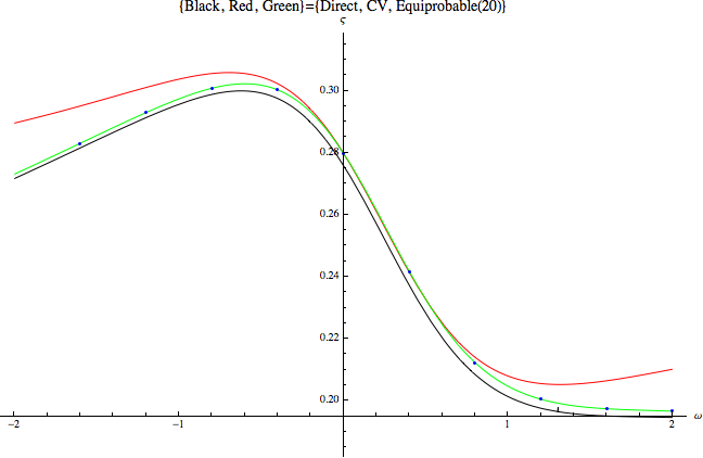
3 Computational Results ¶ Figure 1: Portfolio Share By Method as a Function of ω \omega ω
Figure 1
using the built-in numerical optimizer and maximization functions (the lowest, black, locus), the Campbell-Viceira solution (the highest, red locus)
and an equiprobable approximation using 20 approximation points (green, middle) as well as the solution using the equiprobable approximation
at an evenly-spaced grid of points (blue dots).
Careful examination indicates that the numerical approximation is quite close to the full numerical solution, while the CV approximation diverges substantially from the numerical answer. The tradeoff is that the
equiprobable solution is about 2000 times slower than the CV approximation, while the direct solution is more than 100 times slower
than the equiprobable solution. Depending on the requirements of the problem being examined, these differences in
efficiency can make a tremendous difference in the feasibility of a research project.[2]
Judd, K. L. (1998). Numerical Methods in Economics . The MIT Press. Kopecky, K. A., & Suen, R. M. H. (2010). Finite State Markov-Chain Approximations To Highly Persistent Processes. Review of Economic Dynamics , 13 (3), 701–714. 10.1016/j.red.2010.02.002