Consumption out of Risky Assets - Intertemporal Choice

Consider a consumer with CRRA utility whose only available financial asset has a risky return factor $\RiskyAlt$ which is lognormally distributed, $\log \RiskyAlt_{t+1} \sim \mathcal{N}({\riskyAlt} - \sigma_{\risky}^{2}/2,\sigma_{\risky}^{2})$ .

With market assets $\mRat$ , the dynamic budget constraint is:

{m}_{t+1} = ({m}_{t}-c_{t})\RiskyAlt_{t+1}.

(1)

Start with the standard Euler equation for consumption under CRRA utility:

1 = \Discount \Ex_{t}\left[\RiskyAlt_{t+1}\left(\frac{c_{t+1}}{c_{t}}\right)^{-\CRRA}\right]

(2)

and postulate a solution of the form $c_{t} = \MPC {m}_{t}$ . The guess-and-verify method works here because market resources $m_t$ appear in both numerator and denominator, allowing them to cancel; if labor income appeared in the numerator, this approach would fail.

\begin{aligned} 1 & = \Discount \Ex_{t}\left[\RiskyAlt_{t+1}\left(\frac{\MPC {m}_{t+1}}{\MPC {m}_{t}}\right)^{-\CRRA}\right] \\ & = \Discount \Ex_{t}\left[\RiskyAlt_{t+1}\left(\frac{({m}_{t}-c_{t})\RiskyAlt_{t+1}}{ {m}_{t}}\right)^{-\CRRA}\right] \\ & = \Discount \Ex_{t}\left[\RiskyAlt_{t+1}\left(\frac{(1-\MPC){m}_{t}\RiskyAlt_{t+1}}{ {m}_{t}}\right)^{-\CRRA}\right] \\ & = \Discount \Ex_{t}\left[\RiskyAlt_{t+1}\left((1-\MPC)\RiskyAlt_{t+1}\right)^{-\CRRA}\right] \\ & = \Discount (1-\MPC)^{-\CRRA}\Ex_{t}\left[\RiskyAlt_{t+1}^{1-\CRRA}\right] \\ (1-\MPC)^{\CRRA} & = \Discount \Ex_{t}[\RiskyAlt_{t+1}^{1-\CRRA}] \\ (1-\MPC) & = \left(\Discount \Ex_{t}[\RiskyAlt_{t+1}^{1-\CRRA}]\right)^{1/\CRRA} \\ \MPC & = 1- \left(\Discount \Ex_{t}[\RiskyAlt_{t+1}^{1-\CRRA}]\right)^{1/\CRRA} \end{aligned}

(3)

which (finally) yields an exact formula for $\MPC$ :

\MPC = 1- \left(\Discount \Ex_{t}[\RiskyAlt_{t+1}^{1-\CRRA}]\right)^{1/\CRRA}.

(4)

Since $\log \RiskyAlt_{t+1}^{1-\CRRA} = (1-\CRRA) \log \RiskyAlt_{t+1}$ , fact ELogNormTimes implies that (using the definition $\exp(\bullet) \equiv e^{\bullet}$ ),

\begin{aligned} \Ex_{t}[\RiskyAlt_{t+1}^{1-\CRRA}] & = \exp[(1-\CRRA) ({\riskyAlt} -\sigma_{\risky}^{2}/2)+ (1-\CRRA)^{2} \sigma_{\risky}^{2} /2] \\ & = \exp[(1-\CRRA) {\riskyAlt} -(1-\CRRA)(\sigma_{\risky}^{2}/2) + (1-\CRRA)(\sigma^{2}_{\risky}/2) - \CRRA(1-\CRRA)\sigma_{\risky}^{2}/2] \\ & = \exp[(1-\CRRA) {\riskyAlt} - \CRRA(1-\CRRA)\sigma_{\risky}^{2}/2]. \end{aligned}

(5)

Substituting in (4):

\begin{aligned} \MPC & = 1- \Discount ^{1/\CRRA} \exp\left[\CRRA\left((1/\CRRA - 1){\riskyAlt} - (1-\CRRA)\sigma_{\risky}^{2}/2\right)\right]^{1/\CRRA} \\ & = 1- \Discount ^{1/\CRRA} \exp\left[(1/\CRRA - 1){\riskyAlt} - (1-\CRRA)\sigma_{\risky}^{2}/2\right]. \end{aligned}

(6)

Now use OverPlus and TaylorOne,

\begin{aligned} \Discount^{1/\CRRA} & = \left(\frac{1}{1+\DiscRate}\right)^{1/\CRRA} \\ & \approx 1-\CRRA^{-1}\DiscRate \\ & \approx \exp(-\CRRA^{-1}\DiscRate) \end{aligned}

(7)

which hold if $\CRRA^{-1}\DiscRate$ is close to zero. Substituting into (6) and using ExpPlus and LogEps gives

\begin{aligned} \MPC & \approx 1-(1+\CRRA^{-1}({\riskyAlt}-\DiscRate)-{\riskyAlt}+(\CRRA-1)\sigma_{\risky}^{2}/2) \\ & = {\riskyAlt}-\CRRA^{-1}({\riskyAlt}-\DiscRate) - \left(\CRRA-1\right)(\sigma_{\risky}^{2}/2) \end{aligned}

(8)

which, when $\sigma^{2}_{\risky}=0$ , reduces to the usual perfect foresight formula $\MPC = \riskyAlt - \CRRA^{-1}(\riskyAlt - \DiscRate)$ .

This equation implies the plausible result that as unavoidable uncertainty in the financial return goes up ( $\sigma_{\risky}^{2}$ rises) the level of consumption falls (because $\CRRA>1$ , so $-(\CRRA-1)$ which multiplies $\sigma_{\risky}^{2}$ is negative). The reduction in consumption as risk increases reflects the precautionary saving motive.^[1]

The top figure plots the marginal propensity to consume as a function of the coefficient of relative risk aversion (for both the true MPC and the approximation derived above), under parameter values such that $\DiscRate - \riskyAlt \approx 0$ so that a change in $\CRRA$ does not affect the MPC through the intertemporal elasticity of substitution channel. As intuition would suggest, as consumers become more risk averse, they save more (the MPC is lower; that is, the plotted loci are downward-sloping).

The other way to see the precautionary effect is to examine the effect on the MPC of a change in risk. For a consumer with relative risk aversion of 3, the bottom figure shows that as the size of the risk increases, the MPC $\MPC$ falls.

1Relation Between MPC and Parameters¶

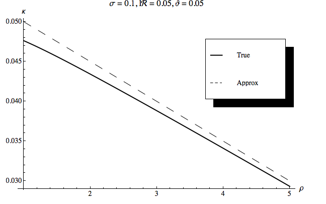
Marginal Propensity to Consume Falls as Relative Risk Aversion \CRRA Rises — Figure 1:Marginal Propensity to Consume Falls as Relative Risk Aversion $\CRRA$ Rises

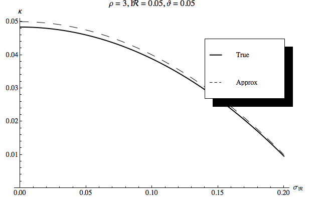
Marginal Propensity to Consume Falls as Risk \sigma Rises — Figure 2:Marginal Propensity to Consume Falls as Risk $\sigma$ Rises

Footnotes¶

It is surprising to note that for a consumer with logarithmic utility, a mean-preserving spread in risk has no effect on the level of consumption (this can be seen by substituting $\CRRA=1$ into (8), which causes the term involving risk $\sigma^{2}_{\risky}$ to disappear from the equation). The reason this is surprising is that intuition suggests that if the consumer’s consumption (and therefore current saving) are unchanged, the increase in uncertainty must constitute a mean-preserving spread in future consumption, which by Jensen’s inequality should yield higher expected marginal utility. The place where this argument goes wrong is that it forgets that the expectation in the Euler equation $\uFunc^{\prime}(c_{t})=\Discount \Ex_{t}[\RiskyAlt_{t+1} \uFunc^{\prime}(c_{t+1})]$ is also affected by a covariance between $\RiskyAlt_{t+1}$ and $\uFunc^{\prime}(c_{t+1})$ ; the case of log utility is the special case where this boils down to a constant times $\Ex_{t}[\RiskyAlt_{t+1}/\RiskyAlt_{t+1}]= 1$ , which is why the expected marginal utility is unaffected by the unavoidable increase in risk. This is yet another reason (if any more were needed) to conclude that logarithmic utility does not exhibit sufficient curvature to plausibly represent attitudes toward risk. ( $\CRRA \geq 2$ seems a plausible lower bound).
↩