The Envelope Theorem and the Euler Equation

This section shows how the Envelope theorem is used to derive the consumption Euler equation in a multiperiod optimization problem with geometric discounting and intertemporally separable utility.

The consumer’s goal from the perspective of date $\tNow$ is to maximize the sum of discounted utilities, where geometric discounting means that utility $n$ periods in the future is weighted by $\Discount^{n}$ :

\max \sum_{n=0}^{\TEnd-\tNow} \Discount^{n} \uFunc(c_{\tNow+n})

(1)

subject to the dynamic budget constraint

{m}_{\tNow+1} = ({m}_{\tNow}-{c}_{\tNow})\Rfree + {y}_{\tNow+1}.

(2)

The problem can be written in Bellman equation form as

\vFunc_{\tNow}({m}_{\tNow}) = \max_{\{{c}_{\tNow}\}} ~\uFunc({c}_{\tNow}) + \Discount \vFunc_{\tNow+1}(({m}_{\tNow}-{c}_{\tNow})\Rfree+{y}_{\tNow+1}).

(3)

The first order condition for (3) can be written as

\begin{aligned} 0 & = \uFunc^{\prime}({c}_{\tNow})+\overbrace{\left(\frac{d {m}_{\tNow+1}}{d {c}_{\tNow}}\right)}^{=-\Rfree} \Discount \vFunc_{\tNow+1}^{\prime}({m}_{\tNow+1}) \\ \uFunc^{\prime}({c}_{\tNow}) & = \Rfree \Discount \vFunc_{\tNow+1}^{\prime}({m}_{\tNow+1}), \end{aligned}

(4)

where the derivative $d {m}_{\tNow+1}/d {c}_{\tNow} = -\Rfree$ follows from (2). We can define a function $\cFunc_{\tNow}({m})$ that returns the ${c}_{\tNow}$ that solves the max problem for any given ${m}_{\tNow}$ . That is, for ${c}_{\tNow}=\cFunc_{\tNow}({m}_{\tNow})$ the first order condition (4) will hold so that

\uFunc^{\prime}(\cFunc_{\tNow}({m}_{\tNow})) - \Rfree \Discount \vFunc_{\tNow+1}^{\prime}(({m}_{\tNow}-\cFunc_{\tNow}({m}_{\tNow}))\Rfree+{y}_{\tNow+1}) = 0.

(5)

Now define a function $\underline{\vFunc}_{\tNow}$ (where the underscore indicates a weak lower bound on value, achieved only when $c$ is chosen optimally):

\underline{\vFunc}_{\tNow}({m}_{\tNow},{c}_{\tNow}) = \uFunc({c}_{\tNow})+\Discount \vFunc_{\tNow+1}(({m}_{\tNow}-{c}_{\tNow})\Rfree+{y}_{\tNow+1})

(6)

with partial derivatives

\underline{\vFunc}^{c}_{\tNow}({m}_{\tNow},{c}_{\tNow}) \equiv \left(\frac{\partial \underline{\vFunc}_{\tNow}}{\partial {c}_{\tNow}}\right) = \uFunc^{\prime}({c}_{\tNow}) - \Rfree\Discount \vFunc_{\tNow+1}^{m}(({m}_{\tNow}-{c}_{\tNow})\Rfree+{y}_{\tNow+1})

(7)

\underline{\vFunc}^{{m}}_{\tNow}({m}_{\tNow},{c}_{\tNow}) \equiv \left(\frac{\partial \underline{\vFunc}_{\tNow}}{\partial {m}_{\tNow}}\right) = \Rfree \Discount \vFunc_{\tNow+1}^{{m}}({m}_{\tNow+1})

(8)

and note that by definition

\vFunc_{\tNow}({m}_{\tNow}) = \underline{\vFunc}_{\tNow}({m}_{\tNow},\cFunc_{\tNow}({m}_{\tNow})).

(9)

The Chain Rule of differentiation tells us that

\vFunc^{\prime}_{\tNow}({m}_{\tNow})\equiv \vFunc_{\tNow}^{{m}}({m}_{\tNow}) \equiv \left(\frac{d \vFunc_{\tNow}}{d {m}_{\tNow}}\right) = \underline{\vFunc}_{\tNow}^{{m}}({m}_{\tNow},\cFunc_{\tNow}({m}_{\tNow})) + \left(\frac{\partial \cFunc_{\tNow}({m}_{\tNow})}{\partial {m}_{\tNow}}\right)\underline{\vFunc}_{\tNow}^{c}({m}_{\tNow},\cFunc_{\tNow}({m}_{\tNow})).

(10)

Here’s the key insight: The assumption that consumers are optimizing means that we will always be evaluating the value function and its derivatives at a ${c}_{\tNow}$ that satisfies the first-order optimality condition (5) (this reasoning would need modification if a liquidity constraint were binding). Thus we have from (7) that

\begin{aligned} \underline{\vFunc}_{\tNow}^{c}({m}_{\tNow},\cFunc_{\tNow}({m}_{\tNow})) & = \uFunc^{\prime}(\cFunc_{\tNow}({m}_{\tNow})) - \Rfree\Discount \vFunc^{\prime}_{\tNow+1}(({m}_{\tNow}-\cFunc_{\tNow}({m}_{\tNow}))\Rfree+{y}_{\tNow+1}) \\ & = 0. \end{aligned}

(11)

This means that the second term in (10) is always equal to zero, so from (8) we obtain

\vFunc^{\prime}_{\tNow}({m}_{\tNow}) = \Rfree \Discount \vFunc_{\tNow+1}^{\prime}({m}_{\tNow+1}).

(12)

Now notice that the RHS’s of (4) and (12) are identical, so we can equate the left hand sides,

\vFunc_{\tNow}^{\prime}({m}_{\tNow}) = \uFunc^{\prime}({c}_{\tNow})

(13)

and since a corresponding equation will hold in period $t+1$ we can rewrite (12) as

\uFunc^{\prime}({c}_{\tNow}) = \Rfree \Discount \uFunc^{\prime}({c}_{\tNow+1}).

(14)

The general principle can be condensed into a rule of thumb by realizing that the Envelope theorem will always imply that the total derivative of a value function with respect to any choice variable must be equal to zero for optimizing consumers (because the first order condition holds). Thus we could have obtained the result immediately by treating ${c}_{\tNow}$ as though it were a constant (that is, treating the problem as though $\cFunc_{\tNow}^{\prime}(m_{\tNow})=0$ ) and taking the derivative of Bellman’s equation with respect to ${m}_{\tNow}$ directly. This leads immediately to the key result:

\begin{aligned} \vFunc_{\tNow}({m}_{\tNow}) & = \uFunc(\cFunc({m}_{\tNow})) + \Discount \vFunc_{\tNow+1}(({m}_{\tNow}-\cFunc_{\tNow}({m}_{\tNow}))\Rfree+{y}_{\tNow+1}) \\ \vFunc_{\tNow}^{\prime}({m}_{\tNow}) & = \Discount \Rfree \vFunc_{\tNow+1}^{\prime}({m}_{\tNow+1}). \end{aligned}

(15)

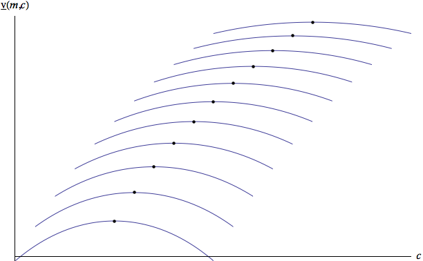
Illustration of the Envelope Theorem at Alternative Values of \mRat — Figure 1:Illustration of the Envelope Theorem at Alternative Values of $\mRat$

The figure illustrates why the Envelope theorem works: when $m$ increases, the increase in attainable utility is approximately the same whether the extra resources are consumed immediately or saved entirely. This is precisely because the first-order condition equates the marginal utility of consumption to the marginal value of saving, so at the optimum the consumer is indifferent at the margin between these alternatives.