Social Security and Capital Accumulation

Consider a household with a 2-period lifetime, whose optimization problem is written in the most general way possible, with the last line reflecting the assumption that no labor income is earned in period 2:

\begin{aligned} \vFunc(\bRat_{1,t}) & = \max_{\{\cRat_{1,t}\}} ~~ \uFunc(\cRat_{1,t}) + \Discount \uFunc(\cRat_{2,t+1}) \\ & \text{s.t.} \\ \yRat_{1,t} & = (\Wage_{1,t}-\taxNetTrans_{1,t}) \\ \aRat_{1,t} & = \yRat_{1,t} - \cRat_{1,t} \\ \yRat_{2,t+1} & = (\Wage_{2,t+1}-\taxNetTrans_{2,t+1}) = -\taxNetTrans_{2,t+1} \\ \cRat_{2,t+1} & = \Rfree_{t+1} \aRat_{1,t}+\yRat_{2,t+1}. \end{aligned}

(1)

Under logarithmic utility, section The Fisher Two-Period Optimal Consumption Problem shows that the solution to this problem is

\cRat_{1,t} = \left(\frac{\yRat_{1,t}+\yRat_{2,t+1}/\Rfree_{t+1}}{1+\Discount}\right).

(2)

The only role of government in this economy is to run a Social Security program. Suppose that initially this economy had no Social Security system and we are interested in the effects of introducing a Pay-As-You-Go Social Security system that is expected to remain a constant size from generation to generation from now on: $\taxNetTrans_{2,t+1} = -\taxNetTrans_{1,t+1}$ while $\taxNetTrans_{1,t+1} = \taxNetTrans_{1,t}$ , so that taxes are greater than transfers when young and transfers are greater than taxes when old.

The effects of Social Security on first period consumption can be seen by writing out explicitly the value for $\cRat_{1,t}$ from equation (2), substituting the definitions of $\yRat_{1,t}$ and $\yRat_{2,t+1}$ :

\begin{aligned} \cRat_{1,t} & = \left(\Wage_{1,t}-\taxNetTrans_{1,t}-\taxNetTrans_{2,t+1}/\Rfree_{t+1}\right)/(1+\Discount) \\ & = \left(\Wage_{1,t}-\underbrace{\rfree_{t+1}\taxNetTrans_{1,t}/\Rfree_{t+1}}_{\text{consume less b/c poorer}}\right)/(1+\Discount) \end{aligned}

(3)

where the expression with the underbrace comes from the effect of introducing a constant-sized PAYG Social Security system in section Generational Accounts and the Government. If taxes paid when young $\taxNetTrans_{1,t}$ are positive (as they are after the introduction of the Social Security system) and the interest rate is positive, the expression with the underbrace is a positive number, and since it is being subtracted from $\Wage_{1,t}$ it is clear that consumption in the first period of life will decline with the introduction of the Social Security system. The reason is that the household is poorer in a lifetime sense: the rate of return on Social Security contributions is lower than the market interest rate.

Does the decline in consumption mean the saving rate rises? No - because saving is after-tax income minus consumption, and net taxes on the young have risen. For saving we have

\begin{aligned} \aRat_{1,t} & = \overbrace{(\Wage_{1,t}-\taxNetTrans_{1,t})}^{\text{Less after-tax income}} - \overbrace{\cRat_{1,t}}^{\text{Lower consumption b/c poorer}} \\ & = (\Wage_{1,t}(1-1/(1+\Discount)) - \taxNetTrans_{1,t}+ [r_{t+1}\taxNetTrans_{1,t}/\Rfree_{t+1}]/(1+\Discount) \\ & = \Wage_{1,t}\left(\frac{\Discount}{1+\Discount}\right)-\taxNetTrans_{1,t}\left(1-\frac{r_{t+1}}{\Rfree_{t+1}(1+\Discount)}\right) \\ & = \Wage_{1,t}\left(\frac{\Discount}{1+\Discount}\right)-\taxNetTrans_{1,t}\left(\frac{\Rfree_{t+1}(1+\Discount)-r_{t+1}}{\Rfree_{t+1}(1+\Discount)}\right) \\ & = \Wage_{1,t}\left(\frac{\Discount}{1+\Discount}\right)-\taxNetTrans_{1,t}\left(\frac{1+\Rfree_{t+1}\Discount}{\Rfree_{t+1}(1+\Discount)}\right). \end{aligned}

(4)

So if $\taxNetTrans_{1,t}>0$ then saving is less than before the introduction of Social Security.

Now consider the implications in a Diamond (1965) OLG model where saving is the source of capital accumulation. Suppose there is no population growth so that

\begin{aligned} K_{t+1} & = \aRat_{1,t} \\ & = \Wage_{1,t}\left(\frac{\Discount}{1+\Discount}\right)-\taxNetTrans_{1,t}\left(\frac{1+\Rfree_{t+1}\Discount}{\Rfree_{t+1}(1+\Discount)}\right) \\ & = (1-\varepsilon)K^{\varepsilon}_{t} \left(\frac{\Discount}{1+\Discount}\right)-\taxNetTrans_{1,t}\left(\frac{1+\Rfree_{t+1}\Discount}{\Rfree_{t+1}(1+\Discount)}\right) \\ & = \mathcal{Q} K^{\varepsilon}_{t} -\taxNetTrans_{1,t}\left(\frac{1+\Rfree_{t+1}\Discount}{\Rfree_{t+1}(1+\Discount)}\right) \end{aligned}

(5)

where $\mathcal{Q}=(1-\varepsilon)\Discount/(1+\Discount)$ as before in the The Diamond OLG Model section.

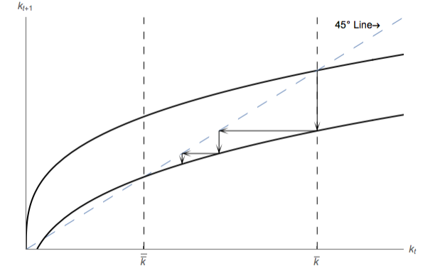
Thus the capital accumulation curve is shifted down (the figure simplifies by assuming a constant downward shift, though strictly speaking $\Rfree_{t+1}$ depends on $k_{t+1}$ ). The dynamics of the introduction of Social Security are captured in the figure, under the assumption that the economy was at its steady-state equilibrium level $\bar{k}$ before the Social Security system was introduced. The effect of introduction is an immediate increase in consumption, as the old generation spends everything it gets and the young generation doesn’t need to do as much retirement saving as before. Over time the economy will converge to its new, lower level of capital $\bar{\bar{k}}$ .

Figure 1:Convergence of OLG Economy After Intro of Social Security

References¶

Diamond, P. A. (1965). National Debt in a Neoclassical Growth Model. American Economic Review, 55(5), 1126–1150.