where ℸ=(1−δ) is the amount of capital left after one period of depreciation at rate δ.[2]et is the value of the profit-maximizing firm: If capital markets are efficient this is the equity value that the firm would command if somebody wanted to buy it.
In words: The marginal cost of an additional unit of investment (the LHS) should be equal to the discounted marginal value of the resulting extra capital (the RHS).
With taxes:(1+jti)P=ℸβet+1k(kt+1), where the LHS is the after-tax marginal cost of investment.
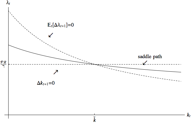
Now suppose that a steady state exists in which the capital stock is at its optimal level and is not adjusting, so costs of adjustment are zero: jt=jt+1=jti=jt+1i=jtk=jt+1k=0.
and the phase diagram is constructed using the Δλt+1=0 locus. In the vicinity of the steady state, we can assume jtk≈0 in which case the Δλt+1=0 locus becomes
which implies (since fk(kt) is downward sloping in kt) that the Δλt=0 locus (that is, the λt(kt) function that corresponds to Δλt=0) is downward sloping.
We now wish to modify the problem in two ways. First, we have been assuming that the firm has only physical capital, and no financial assets. Second, we have been assuming that the manager running the firm only cares about the PDV of profits; suppose instead we want to assume that the firm is a small business run by an entrepreneur who must live off the dividends of the firm, and thus they are maximizing the discounted sum of utility from dividends u(ct) rather than just the level of discounted profits. (Note that we designate dividends by ct; dividends were not explicitly chosen in the q-model version of the problem, because the Modigliani-Miller theorem says that the firm’s value is unaffected by its dividend policy).
We call the maximizer running this firm the “entrepreneur.” The entrepreneur’s level of monetary assets mt evolves according to
That is, next period the firm’s money is next period’s profits plus the return factor on the money at the beginning of this period, minus this period’s investment and associated adjustment costs, minus dividends paid out (which, having been paid out, are no longer part of the firm’s money).
This holds because maximizing with respect to mt+1 (subject to the accumulation equation) is equivalent to maximizing with respect to the components of mt+1.
Since behavior (for either a firm manager or a consumer) is determined by Euler equations, and the Euler equations for both consumption and investment are identical in this model to the Euler equations for the standard models, there is no observable consequence for investment of the fact that the firm is being run by a utility maximizer, and there is no observable consequence for consumption of the fact that the consumer owns a business enterprise with costly capital adjustment.
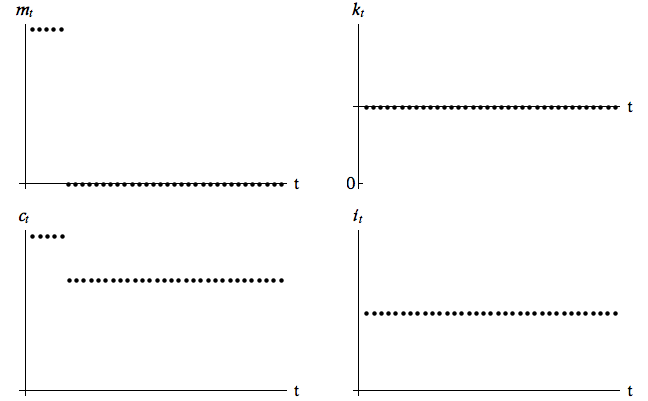
Now consider a firm of this kind that happens to have arrived in period t with positive monetary assets mt>0 and with capital equal to the steady-state target value kt=kˇ.
Suppose that a thief steals all the firm’s monetary assets.
The consequences for the firm are depicted in Figure 2.
Figure 2:Impulse response to a negative shock to mt (monetary assets stolen).
Dividends follow a random walk. Thus, there is a one-time downward adjustment to the level of dividends to reflect the stolen money. Thereafter dividends are constant, as are monetary assets (which are constant at zero forever).
The theft of the money has no effect on investment or the capital stock, because the firm’s investment decisions are made on the basis of whether they are profitable and the theft of the money has no effect on the profitability of investments.
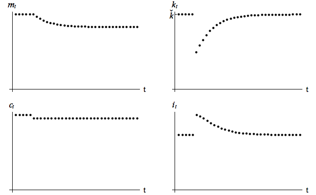
Figure 3:Impulse response to a negative shock to kt (capital destroyed by meteor).
Again, because dividends follow a random walk, what the firm’s managers do is to assess the effect of the meteor shock on the firm’s total value and they adjust the level of dividends downward immediately to the sustainable new level of dividends. Thereafter there is no change in the level of dividends.
Investment is more complicated. The firm’s capital stock is obviously reduced below its steady-state value by the meteor, so there must be a period of high investment expenditures to bring capital back toward its steady state. However, the firm started out with monetary assets of zero. Therefore the high initial investment expenditures will be paid for by borrowing, driving the firm’s monetary assets to a permanent negative value (the firm goes into debt to pay for its rebuilding). Gradually over time the capital stock is rebuilt back to its target level, and investment expenditures return to zero (or the level consistent with replacing depreciated capital).
where Ψ is the firm’s productivity and ℓ is the labor supplied by the entrepreneur (assumed equal to 1).
The policy functions are obtained using the method of reverse shooting, which is based on recovering for a given kt+1 and et+1(kt+1) the values of kt, it and et(kt) consistent with the first order conditions and transition equations.
The reverse-shooting equation for capital comes from a combination of the dynamic budget constraint and the Euler equation. For convenience defining
With the values of it and jt obtained from these reverse-shooting equations, the reverse-shooting equation for value is very simple: It is the Bellman equation
while the steady-state value of λ comes from substituting kˇ into (14). Steady-state value is straightforward to compute, given that in the steady state the capital stock and amount of investment are constant:
The reverse shooting routine starts its backwards iterations from a kt^ level very close to the steady state of the model and, as discussed in the methodological appendix to the TractableBufferStock section, the accuracy of the solution is improved if we approximate it^ with a first order Taylor expansion using the derivative of investment at the steady state:
where the ˇ identifies variables at the steady state and ϵ is the deviation from the steady state. iˇk is computed by differentiating the Euler equation with respect to k:
because this corresponds to the solution to a perfect foresight consumption problem in which the consumer has monetary resources mt and net nonmonetary financial resources et(kt)−ft (see the Consumption Under Perfect Foresight and CRRA Utility).
The model can include corporate taxes. With taxes, additional parameters are: τ (tax rate on corporate earnings), τ=1−τ (portion of earnings untaxed), πt=f(kt)τ (after tax revenues), ζ (investment tax credit), P=ζ=1−ζ (cost of 1 unit of investment after ITC), and ξt=(it+jt)P (after-tax expenditures on investment).
There are some small differences between the formulation of the model here and in the The Abel (1981)-Hayashi (1982) Marginal q Model. Here, investment costs are paid at the time of investment and the depreciation factor applies to (kt+it) rather than just kt. These changes simplify the computational solution without changing any key results.
The slight modification to the cost-of-adjustment function (relative to the formulation in the The Abel (1981)-Hayashi (1982) Marginal q Model) reflects the changed timing of depreciation in (2) compared to the corresponding equation in qModel. In the continuous-time limit the two equations become the same, but the formulation here makes the representation of the problem slightly more transparent in the discrete-time computer code. The code also includes the parameters P and τ (respectively the investment cost after the Investment Tax Credit and the untaxed portion of earnings) in order to study the impact of tax policies. Both parameters are however assumed equal to 1 and thus the equations in the code are equivalent to the simpler ones described in this section.