This section presents a discrete-time version of the Abel Abel (1981)-Hayashi Hayashi (1982) marginal model of investment.
A corresponding Jupyter Notebook implements numerical solutions to the model using HARK and dolo.
1Definitions
To simplify some algebra, we assume that a unit of investment purchased in period does not become productive until ; the cost at reflects the present discounted value of the period- price of capital.[1]
Adjustment costs are priced the same way.[2] We repeatedly make approximations motivated by results from the continuous-time model; the key approximation will be the usual calculus result that if and are “small” then can be approximated by zero. (We will call this fact SmallSmallZero in the MathFactsList.)[3]
| Symbol | Definition | |
|---|---|---|
| - | Firm’s capital stock at the beginning of period | |
| - | Gross output excluding investment and adjustment costs | |
| - | Tax rate on corporate earnings | |
| - | = Portion of earnings remaining after corporate tax | |
| - | After tax revenues | |
| - | Investment in period (affects capital stock in period ) | |
| - | AdJustment costs incurred in period ; smooth and convex | |
| - | Discount factor for future profits (inverse of interest factor) | |
| - | Investment tax credit (ITC) | |
| - | = Cost of investment after ITC |
With time-varying price: denotes the price of one unit of investment, and is the effective after-tax price of 1 unit of investment.
With constant price: When , the after-tax price simplifies to .
| Symbol | Definition | |
|---|---|---|
| - | Total after-tax period- spending on investment (with time-varying price) | |
| - | Total after-tax period- spending on investment (with constant price) | |
| - | Depreciation rate | |
| - | Depreciation factor | |
| - | Adjustment cost parameter |
2The Problem
The model assumes that firms maximize the net profits payable to shareholders, definable as the present discounted value of after-tax revenues after subtracting off costs of investment:
Next period’s capital is what remains of this period’s capital after depreciation, plus current investment:[4]
If capital markets are efficient, will also be the stock market value (“equity” is the mnemonic) of the profit-maximizing firm because it is precisely the amount that a rational investor will be willing to pay if they care only about discounted after-tax income derived from owning (a share of) the firm.
We can simplify by thinking about the firm’s shareholders as the suppliers of physical capital, not just financial capital. In this interpretation, represents not just the value of the physical machinery owned by the firm, but also the number of shares of stock outstanding in the firm. We can think of the firm in this way if we suppose that every time the firm purchases new physical capital, it does so by issuing new shares at a price equal to the marginal valuation of the firm’s capital stock, purchasing the unit of capital at the price given by the after-tax cost of that capital (and after paying any associated adjustment costs).[5]
The Bellman equation for the firm’s value can be derived from
which is equivalent to
and defining as the derivative of adjustment costs with respect to the level of investment,[6] the first order condition for optimization with respect to (or, equivalently, ) is
Thus: The PDV of the marginal cost (after tax, including adjustment costs) of an additional unit of investment should match the discounted expected marginal value of the resulting extra capital. (Recall that investment performed today is paid for tomorrow at price so today’s cost is .)
Recalling that , the The Envelope Theorem and the Euler Equation theorem for this problem can be used on either (3) or (4):
and equivalently for period so that (5) can be rewritten as the Euler equation for investment,
It will be useful to define the net investment ratio as the Greek letter (the absence of a dot distinguishes from the level of investment ),
which measures how much investment differs from the proportion necessary to maintain the capital stock unchanged. It has derivatives
We now specify a convex (quadratic) adjustment cost function centered around the depreciation rate . The rationale for this centering is that when (investment exactly replaces depreciated capital), the firm is simply maintaining its existing capital stock and incurs no adjustment costs. Adjustment costs arise only when the firm deviates from this “replacement investment” benchmark:
with derivatives (using (9) to simplify)
so the Euler equation for investment (7) can be written
To begin interpreting this equation, consider first the case where the costs of adjustment are zero, . In this case and the Euler equation reduces to
Simplifying further, suppose that capital prices are constant at and the ITC is unchanging so that the after-tax price of capital is constant at . Then since , the equation becomes
This says that the cost of buying one unit of capital, , is equal to the opportunity cost in lost interest plus the value lost to depreciation, , which must match the (after-tax) payoff from ownership of that capital. This corresponds exactly to the formula for the equilibrium cost of capital in the The Hall-Jorgenson Model of Investment model: In the presence of an investment tax credit at rate , the after-tax price of capital is , and the firm will adjust its holdings of capital to the point where
Now define as the marginal value to the firm of ownership of one more unit of capital at the beginning of period ; using this definition, the envelope condition can be written
where the last approximation uses in the form . Equation (16) can be rearranged as
This equation can best be understood as an arbitrage equation for the share price of the company if capital markets are efficient.[7] The first term on the RHS is the flow of income that would be obtained from putting the value of an extra unit of capital in the bank. The term in brackets is the flow value of having an extra unit of capital inside the firm: Extra after-tax revenues are measured by the first term, the second term accounts for the effect of the extra capital on costs of adjustment, and the final term reflects the cost to the firm of the extra depreciation that results from having more capital.
Think first about the case, in which the firm’s value, share price, and size will be unchanging because the marginal value of capital inside the firm is equal to the opportunity cost of employing that capital outside the firm (leaving it in the bank). If these two options yield equivalent returns, it is because the firm is already the “right” size and should be neither growing nor shrinking.
Now consider the case where , because
This says that an extra unit of capital is more valuable inside the firm than outside it, which means that 1) is above its steady-state value; 2) the firm will have positive net investment; and 3) the firm’s share value will be falling over time (because the level of its share value today is high, reflecting the fact that the high marginal valuation of the firm’s future investment has already been incorporated into ).[8]
Now define “marginal ” as the value of an additional unit of capital inside the firm divided by the after-tax purchase price of an additional unit of capital,[9]
The investment first order condition (5) implies
which constitutes the implicit definition of a function
and notice that this implies
At a value of , investment takes place at a rate exactly equal to the depreciation rate ()
The investment ratio is monotonically increasing in ()
The strength with which is related to depends on the magnitude of adjustment costs ()
3Phase Diagrams
3.1Dynamics of 
The capital accumulation equation can be rewritten as
3.2Dynamics of 
To construct a phase diagram involving , we need to transform our equation (16) for the dynamics of into an equation for the dynamics of . As a preliminary, define the proportional change in the after-tax price of capital as
Recalling that , dividing both sides of (16) by yields
Now assuming that , , , and are all “small” so that their interactions are approximately 0, we have
Simplifying further, if the ITC is unchanging, and the pretax price of capital is unchanging at , and , equation (25) becomes
where
combines the effects of the corporate tax and the investment tax credit into a single tax term. Its inverse, , appears in subsequent analysis where it is convenient to express the tax-adjusted marginal product of capital as .
3.3Results
Figure Figure 2 presents two phase diagrams, one for and and one for and .
For most purposes, diagram is simpler, because our facts about the function imply that the locus is always a horizontal line at . This is because always corresponds to the circumstance in which the value of a unit of capital inside the firm, , matches the after-tax cost of a unit of capital, ; is the only value of at which the firm does not wish to change size ().
The slope of the locus is easiest to think about near the steady state value of where we can approximate .
Pick a point on the locus. Now consider a value of that is slightly larger. From (26), at the initial value of we would have . Thus, the value of corresponding to must be one that balances the higher by a higher value of , which is to say a lower value of . This means that higher will be associated with lower so that the locus is downward-sloping.
For appropriate choices of parameter values the problem satisfies the usual conditions for stability and will therefore have a saddle path solution, as depicted in the diagram.
The diagram is virtually indistinguishable from the diagram; the only difference is that the locus is located at the point (i.e. the marginal value of investment is equal to the price of a unit of investment). The distinction between the diagrams reflects the fact that an increase in the investment tax credit will result in a rise in the steady-state value of which implies a fall in the pretax marginal product of capital.
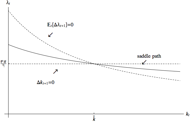
Figure 1:Phase Diagram for
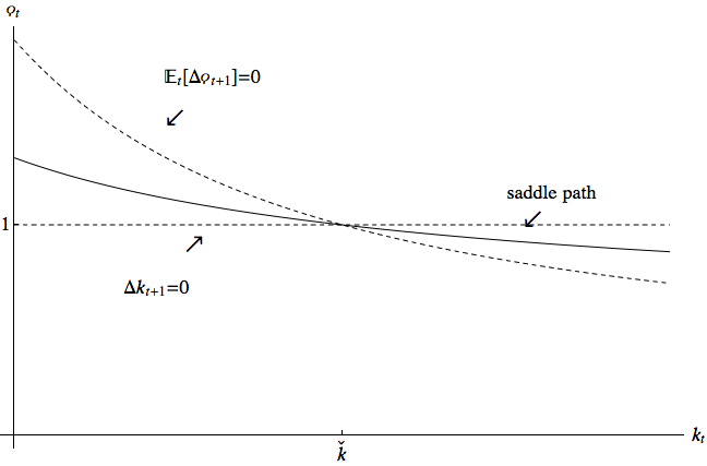
Figure 2:Phase Diagram for
4Dynamics
4.1Steady State
The key to understanding the model’s dynamics (as, really, with all infinite horizon models) is to figure out the steady state toward which it is heading, then to work out how it gets there. The key to the steady state, in turn, is that the capital stock will eventually reach a point where .
4.2A Positive Shock to Productivity
Suppose that the production function for the firm suddenly, permanently, and unexpectedly improves; specifically, leading up to period the firm was in steady state, but in periods and beyond the production function will be for some where and indicate the production functions before and after the increase in productivity.
Note first that none of the tax terms has changed, and in the long run there is nothing to prevent the firm from adjusting its capital stock to the point consistent with the new level of productivity and then leaving it fixed there so that . Thus (26) implies that at the new steady state we will have which implies , since the steady state value of never changes: . That is, with higher productivity, the equilibrium capital stock is larger, but the equilibrium tax adjusted marginal product of capital is the same.
Obviously in order to get from an initial capital stock of to a larger equilibrium capital stock of the firm will need to engage in investment in excess of the depreciation rate, incurring costs of adjustment. In the absence of a change in the environment, expected costs of adjustment will always be declining toward zero, because the firm’s capital stock will always be moving toward its equilibrium value in which those costs are zero.
So we can tell the story as follows. Suppose that leading up to period the firm was in its steady-state. When the productivity shock occurs, jumps up. had been zero (because the firm was at steady state), but now the firm wishes it had more capital because extra capital would reduce future adjustment costs (the firm knows that its old steady-state capital stock is now too small, so it will have to be engaging in for a while), so becomes negative (that is, the firm knows that having more capital will reduce the adjustment costs associated with the higher investment that it will be undertaking). The combination therefore becomes a larger positive number, so at the initial level of the RHS of (26) would imply less than zero, so the new locus must be higher (because the equilibrating value of is higher for any ). The saddle path is therefore also higher. So , and therefore , jump up instantly when the new higher level of productivity is revealed, corresponding also to an immediate increase in the firm’s share price (the marginal valuation of an additional unit of capital), since has not changed.
The phase diagrams with the saddle paths before and after the productivity increase together with the impulse response functions would be plotted here.
4.3A Permanent Tax Cut
Again starting from the steady state equilibrium, suppose unexpectedly and permanently decreases, which could happen because of a cut in corporate taxes or an increase in the ITC. Equation (26) implies that in steady state
Dynamically, the story is as follows. Equation (26) implies that following the tax change the locus must be higher because at any given the term is a larger negative number, while at the initial the term is also now negative; so the locus shifts up.
In contrast to the case with a productivity shock, the equilibrium marginal product of capital will be lower than before. Arbitrage equalizes the after-tax marginal product of capital with the interest rate, but with a lower tax rate, that equilibration will occur at a higher level of capital.
Notice that the qualitative story is the same whether the change in is due to a permanent reduction in the corporate tax rate (increase in ) or a permanent increase in the investment tax credit (reduction in ). In either case, and investment jump upward at time and then gradually decline back downward (though the equilibrium level of investment is higher than before the change).
There is, however, one interesting distinction between a decrease in due to a reduction in corporate taxes and a decrease caused by an increase in . Since , an increase in reduces and therefore reduces the equilibrium value of , while a change in has no effect on equilibrium . This reflects a subtle distinction. is the after-tax marginal value of extra capital, and the equilibrium in this model will occur at the point where that marginal value is equal to the marginal cost. Changing changes that marginal cost, so it changes the equilibrium after-tax marginal value. Changing does not change the marginal cost of capital, so the equilibrium after-tax marginal value of capital is unchanged. The marginal product of capital is lower after a tax cut (equilibrium is smaller), but that is exactly counterbalanced by the larger value of so that is unchanged in the long run by the change in .
The phase diagrams with the saddle paths before and after the corporate tax reduction and the ITC increase, together with the impulse response functions, would be plotted here. Note that the saddle path actually jumps downward after the ITC increase. This is not an error; rather, recall that reflects marginal value of a unit of capital inside the firm, and recall that the price of purchasing that capital has gone down. Remembering that we are assuming that capital can move in and out of the firm, this has the surprising consequence that, for the original owners of the firm, the ITC is bad news because it means that the capital they own has a lower value (its value is ultimately tied to the price of capital, which has gone down). For a potential new shareholder, the investment tax credit means that you can obtain ownership of a share of the firm’s capital by buying the capital at the ITC-discounted price, paying the adjustment costs, then giving the capital to the firm. Thus, the ITC has the effect of increasing the absolute value of a dollar of money relative to the value of a unit of capital inside the firm. So in this special case, you should think of the ITC as something that provides a discount to purchasing shares or capital . While the new saddle path for is lower than the old one, that does not reflect the adjustment for the fact that the new capital is being purchased at a cheaper price. The dynamics of , in this case, are more intuitive than those of : unambiguously increases, reflecting the fact that the value of capital to the firm exceeds its new (cheaper) cost.
In sum: In terms of effects on capital, the outcome from a corporate tax cut and an ITC tax cut are similar, but the analytics of are different, because the former affects the after-tax interest rate while the latter affects the after-tax cost of capital.
4.4A Future Shock to Productivity
Now consider a circumstance where the firm knows that at some date in the future, , the level of productivity will increase so that for .
The long run steady state is of course the same as in the example where the increase in productivity is immediately effective.
To determine the short run dynamics, notice several things. First, there can be no anticipated big jumps in the share price of the firm (the marginal productivity of capital inside the firm). Thus, if the productivity jump occurs in period and the time periods are short enough, we must have
But because the equilibrium capital stock is larger, we know that and will stay negative thereafter (asymptoting to zero from below). This reflects the fact that if you know you will need higher capital in the future, the most efficient way to minimize the cost of obtaining that capital is to gradually start building some of it even before you need it, rather than trying to do it all at once. Note further that before period the model behaves according to the equations of motion defined by the problem under the parameter values,[10] while at and after it behaves according to the new equations of motion.
Putting all this together, the story is as follows. Upon announcement of the productivity increase, jumps to the level such that, evolving exactly according to its equations of motion, it will arrive in period at a point exactly on the saddle path of the model corresponding to the equations of motion. Thereafter it will evolve toward the steady state, which will be at a higher level of capital than before, , because the greater productivity justifies a higher equilibrium capital stock.
Thus, jumps up at time , evolves to the northeast until time , and thereafter asymptotes downward toward the same equilibrium value it had originally before the productivity change. Since has not changed, the dynamics of and are the same as those of .
4.5A Future Increase in the ITC
Consider now the consequences if a surprise increase in the investment tax credit is passed at date that will become effective at date .
Inspection of (26) might suggest that the effects of a future tax cut would be identical to the effects of a future increase in , since the terms enter multiplicatively via . And indeed, with respect to the dynamics of the two experiments are basically the same. And of course the steady-state value of is always equal to one.
During the transition, however, has interesting dynamics. From periods to , the ITC does not change, leaving and the after-tax marginal product of capital unchanged, and so the dynamics of are basically the same as those of But between and , cannot jump but does jump, which implies that must jump (so there is a predictable change in ).
Dynamics of investment are determined by dynamics of , so the path of is: At , a discrete jump up; between and , a gently rising path; between and , an upward jump; and after , a path that asymptotes downward toward the steady state level of investment.
The steady-state effects on are of course determined by the same considerations as apply to the unanticipated tax cut, so they depend on whether the tax change is a drop in or an increase in .
5More Figures
Figures for a variety of other experiments have been constructed using the notebook. Such figures are contained in the “Figures” subdirectory.
This assumption simplifies many of the expressions that arise in the discrete-time framework; in continuous time the model presentation is simpler, but is hard to map the continuous-time theory into a transparent computational solution like the one that accompanies these notes.
To avoid arbitrage opportunities, assume that if you claimed an investment tax credit on a unit of investment in period , then if you resell the portion that remains after depreciation in a future period, you must repay the ITC corresponding to the remaining capital. Actual tax treatment of depreciation is too complicated be worth incorporating into the model; these assumptions capture the core of it.
We neglect tax depreciation because, as shown in the The Hall-Jorgenson Model of Investment section, it matters only insofar as it affects the cost of capital; since the investment tax credit has a more transparent and direct effect on the cost of capital, including tax depreciation would add complication without adding any fundamental insights to the analysis. In the perfect foresight framework analyzed here, any attempt to analyze the effects of changes in tax depreciation should be translatable into an equivalent modification to the ITC. See House & Shapiro (2008) for elaboration.
The software archive that produces the figures for this section makes a slightly different assumption about the timing of depreciation: The timing choice makes no qualitative and very little quantitative difference, but the alternative specification is slightly better for computational reasons.
We implicitly assume in the following derivations that the structure of the function is appropriate to our needs; later we will define a specific that will always work, but here we want to leave the structure of the function general.
This interpretation requires the assumption (made above) that the number of shares outstanding for the firm is equal to the number of units of capital the firm has; this is justifiable by the assumption that in an efficient capital market shares can always be issued or repurchased at an implicit interest rate corresponding to the riskless rate.
The case with rising share prices is symmetric.
The variable naming conventions here differ subtly from those in Romer (2011): what we call Romer calls . Romer also makes different assumptions about the production function.
Strictly speaking, this is not true, because will now differ from the value associated with the initial problem. For purposes of analyzing problems of this kind (announced future changes in parameters) we will neglect the effects of the path of on the equations of motion. Except under extreme circumstances, this should not change the qualitative results of the analysis, and doing anything else would require a very intricate analysis. This treatment is admittedly a bit inconsistent, since in the case under consideration it is precisely the change in that motivates the firm to start adjusting its capital stock before the productivity change comes into effect; effectively, we are taking into account the effect of on the level of before period while neglecting its effects on ’s dynamics during this interval. C’est la vie.
- Abel, A. B. (1981). A Dynamic Model of Investment and Capacity Utilization. Quarterly Journal of Economics, 96(3), 379–403.
- Hayashi, F. (1982). Tobin’s Marginal Q and Average Q: A Neoclassical Interpretation. Econometrica, 50(1), 213–224. 10.2307/1912538
- House, C. L., & Shapiro, M. D. (2008). Temporary Investment Tax Inventives: Theory with Evidence from Bonus Depreciation. American Economic Review, 98(3), 737–768.
- Romer, D. (2011). Advanced Macroeconomics (Fourth). McGraw-Hill/Irwin.