Consider a Ramsey economy in which the capital stock
cannot be freely adjusted; instead, as in the model of investment,
capital is subject to quadratic costs of adjustment.
The dynamic budget constraint is
where for analytical simplicity we neglect capital depreciation (though the illustrative figures below show results of a model that properly includes depreciation) and the cost-of-adjustment function takes the form
for some constant , so that the cost of adjustment incurred in period
is given by
A social planner is assumed to maximize the discounted sum of
utility from consumption , where the utility function is CRRA, .
The social planner’s problem can be rewritten in the form of a Bellman equation,
Because (given ), choosing is equivalent to choosing ,[1]
the problem as:
The first order condition is found by setting the derivative w.r.t. to zero:
The envelope theorem tells us that the marginal value of capital does not depend on its effect on the investment policy function :
(where notice that does not have the simple interpretation of a share price as in The Abel (1981)-Hayashi (1982) Marginal q Model because here it involves ).
Substituting period ’s version of (7) into (6) allows us to rewrite the Euler equation in the form:
This economy reduces to a standard Ramsey model when the cost of
adjustment parameter is set to , because all the
terms disappear so that the interest factor becomes the usual
{math}\Rfree_{t+1}=\digamma^{\prime}(\kap_{t+1}) = 1 + \fFunc^{\prime}(\kap_{t+1}). The presence of adjustment costs does
not change the steady state of the model (because in steady state,
adjustment costs are zero), but reduces the speed of convergence
toward that steady state. This can be seen by considering the policy
functions plotted in Figure 1, where the
solid lines reflect the solution to a model with (the
standard Ramsey model) while the dashed lines reflect a model with a
high cost of adjustment (the ‘-Ramsey’ model).
The differences between the solid and the dashed loci indicate that a
faster rate of convergence to the steady state requires a high level
of below the steady state at which and
low level of when is above . Higher
adjustment costs work against fast convergence, since, when is
below the steady state (and positive investment is needed to increase
toward , adjustment costs reduce investment,
while they increase investment (making it less negative) when
is above the equilibrium. In both cases, the difference occurs because
because adjusting capital involves convex costs, and thus it is
optimal to proceed slowly in moving the capital stock to minimize
those costs. Interestingly, even though the optimal choices of
investment and consumption change quite substantially in the model
with a larger adjustment cost parameter, the actual size of costs of
adjustment borne is quite modest (the dashing line for is
barely distinguishable from the horizontal axis except very far from
the steady state). This tells us that even if the observed costs paid
are not very large, those costs can have a large effect in
changing behavior away from the frictionless optimum.
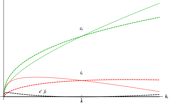
Figure 1:Solid Loci: Standard Ramsey Model; Dashed: With Costs of Adjustment
Increasing the desired degree of consumption smoothing, captured by
the coefficient of relative risk aversion , leads to similar
implications. Figure 2 shows that a higher
(the dashed loci), implies again lower
investment below the steady state and higher above it. This is now
caused by a low intertemporal elasticity of substitution: if the
economy falls below steady state, a larger implies that the
representative agent is less willing to cut consumption in order to
boost investment and quickly return to the steady state. Similarly,
the increase in consumption above the steady state is more moderate,
thus leading to a smaller reduction in investment and a more gradual
return to equilibrium.
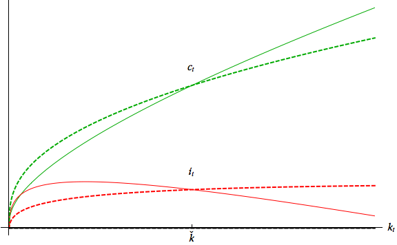
Figure 2:Higher (Dashed Loci) Has a Similar Effect to Adjustment Costs
By comparing the policy functions, we have thus seen that either an
intensified consumption smoothing motive (higher ) and or a stronger investment
smoothing motive (higher ) have similar implications: they
restrain sharp adjustments to consumption and investment, thus slowing
down the speed of convergence to the steady state.
We now consider the responses of the model to several shocks, starting
from steady state. Figure 3 shows the
economy’s dynamics following the destruction of part of the capital
stock. In the standard Ramsey model (black), this leads to
an increase in the marginal productivity of capital which boosts
investment. In the model with adjustment costs (red), the
level of investment actually falls. This is because costs of
adjustment are assumed to be relative to the size of the capital
stock, and with a shrunken capital stock the original level of
investment would incur very large costs of adjustment. Investment
therefore drops to a level that is large relative to the (shrunken)
capital stock but nevertheless smaller than its initial level. Even this lower
investment level, though, is large relative to the new lower level of the
capital stock, and so the capital stock rises back toward the original
equilibrium – just more slowly than in the frictionless model.
Consumption drops due to the negative wealth effect and
the need to finance investment. But since investment is lower initially in
the model with investment costs, consumption can be higher initially (the first
red consumption dot is above the first black one, post-shock).
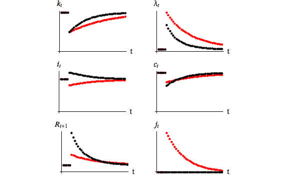
Figure 3:Impulse response functions to 50% destruction of the capital stock
(standard Ramsey) in black; (-Ramsey) in red
Figure 4 shows the dynamics triggered by an
increase in patience, captured by a permanent rise in
. The most striking difference is in the interest factor .
In the Ramsey model with no investment costs, the interest rate is simply
the marginal product of capital. Here, it must also take account of costs
of adjustment. Since costs of adjustment are high when the economy is
trying to change the size of the capital stock, the interest rate is lower.
This result is interesting because one problem with using the Ramsey model
for studying business cycle dynamics is that the aggregate capital stock
barely moves at all over such a short time period as a business cycle,
so the non- Ramsey model has no hope of matching empirical interest rate fluctuations.
Adding costs of adjustment allows much bigger movements in and
thus gives the model a fighting chance.
Given the lower interest rate (and its implications through the
consumption Euler equation), the growth rate of consumption after the
increase in patience will be less than in the standard Ramsey model.
Even though consumption drops less, rises more. Recall
that is a composition of the marginal utility of
consumption and the “share price” of ownership of a unit of capital.
The extra rise in reflects the fact that the existing
capital is more valuable in a period when the rate of investment will
be high (going forward), so the market value of a unit of
“installed” capital rises to above the purchase price of a unit of
capital (which is always 1). This can be interpreted as a boom in
asset prices.
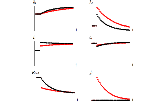
Figure 4:Impulse responses to an increase in patience (higher )
Black: Ramsey; Red: -Ramsey
Finally, we consider in Figure 5
the responses to an increase in the
depreciation rate. This reduces the marginal product of capital and
consequently the desired level of capital. In the Ramsey model,
investment contracts, freeing resources for consumption which
temporarily increases. The economy converges to an equilibrium with
lower capital (at which the marginal productivity returns to its
initial level), lower consumption and investment. In the model with
adjustment costs, consumption initially contracts because investment
actually rises (since the cost of adjustment is defined as
relative to the amount of depreciation, which has suddenly
increased). Because investment increases initially, consumption
falls a bit. As always, however, the economy with costs of
adjustment eventually asymptotes to the same equilibrium as the
frictionless economy.
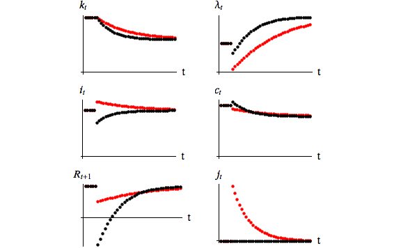
Figure 5:Impulse response functions to an increase in depreciation (higher )