Learning Objectives
TODO: Add learning objectives for this chapter. The sections below provide a starting template:
13.1 TODO: objective for “Pooling Independent Cross Sections across Time”
13.2 TODO: objective for “Policy Analysis with Pooled Cross Sections”
13.3 TODO: objective for “Two-Period Panel Data Analysis”
13.4 TODO: objective for “Policy Analysis with Two-Period Panel Data”
13.5 TODO: objective for “Differencing with More Than Two Time Periods”
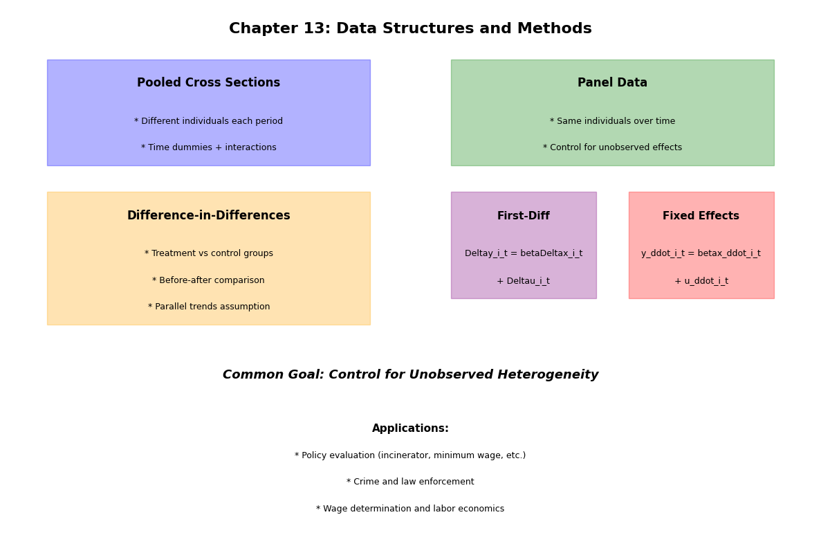
Panel data methods exploit the time dimension of repeated observations to address fundamental identification challenges in empirical research. This chapter develops techniques for analyzing pooled cross-sectional data and longitudinal panel data, establishing how the temporal structure enables researchers to control for unobserved heterogeneity and obtain more credible causal estimates than pure cross-sectional analysis permits.
The presentation proceeds hierarchically from pooled cross sections to sophisticated panel data estimators. We begin with pooling independent cross sections across time to analyze policy changes through difference-in-differences approaches (Section 13.1-13.2), introduce the structure and advantages of true panel data tracking the same units over time (Section 13.3), develop first-differencing methods that eliminate time-invariant unobserved factors in two-period panels (Section 13.4), and extend these techniques to fixed effects estimation accommodating multiple time periods (Section 13.5). Throughout, we implement methods using Python’s linearmodels package and demonstrate applications to labor economics, education policy evaluation, and crime deterrence analysis.
# Import required libraries
import matplotlib.pyplot as plt
import numpy as np
import pandas as pd
import statsmodels.formula.api as smf
import wooldridge as wool
from IPython.display import display
from linearmodels import FirstDifferenceOLS, PanelOLS

plt.style.use("theme.mplstyle")
13.1 Pooling Independent Cross Sections across Time
When we have independent random samples from the same population at different points in time, we can pool these cross sections to increase sample size and statistical power. This approach is particularly useful when individual samples are small.
Key Features of Pooled Cross-Sectional Data
Independence: Different individuals are sampled in each time period
Time dummies: We typically include year or time period indicators
Increased precision: Larger sample size leads to smaller standard errors
Temporal variation: Allows us to study changes over time
The basic pooled cross-sectional model is:
where:
indexes individuals and indexes time periods
are time period dummy variables
capture time effects (shifts in intercept)
Example 13.2: Effect of Education on Wages Across Time
We’ll analyze how the return to education changed between 1978 and 1985 using the Current Population Survey (CPS) data.
# Load the CPS data for 1978 and 1985
cps78_85 = wool.data("cps78_85")

# Display basic information
print("Dataset shape:", cps78_85.shape)
print("\nVariable names:", cps78_85.columns.tolist())
print("\nSummary statistics:")
display(cps78_85.describe())
Dataset shape: (1084, 15)
Variable names: ['educ', 'south', 'nonwhite', 'female', 'married', 'exper', 'expersq', 'union', 'lwage', 'age', 'year', 'y85', 'y85fem', 'y85educ', 'y85union']
Summary statistics:
# Check the distribution of observations across years
year_counts = cps78_85["year"].value_counts().sort_index()
print("Observations by year:")
print(year_counts)
Observations by year:
year
78 550
85 534
Name: count, dtype: int64
Now let’s estimate a model with interactions to see how returns to education and the gender wage gap changed over time:
# Create year dummy (1985 = 1, 1978 = 0)
cps78_85["y85"] = (cps78_85["year"] == 85).astype(int)

# Estimate model with interaction terms
# The formula y85*(educ+female) expands to:
# y85 + educ + female + y85:educ + y85:female
model_interact = smf.ols(
    formula="lwage ~ y85*(educ+female) + exper + I((exper**2)/100) + union",
    data=cps78_85,
)
results_interact = model_interact.fit()

# Create formatted results table
results_table = pd.DataFrame(
    {
        "Coefficient": results_interact.params,
        "Std. Error": results_interact.bse,
        "t-statistic": results_interact.tvalues,
        "p-value": results_interact.pvalues,
    },
)
print("Pooled Regression with Interaction Terms")
print("=" * 70)
display(results_table.round(4))
print(f"\nR-squared: {results_interact.rsquared:.4f}")
print(f"Observations: {int(results_interact.nobs)}")
Pooled Regression with Interaction Terms
======================================================================
R-squared: 0.4262
Observations: 1084
# Interpretation of key coefficients
print("INTERPRETATION OF KEY RESULTS:")
print("=" * 70)

# Base return to education in 1978
base_educ = results_interact.params["educ"]
print(f"\n1. Return to Education in 1978: {base_educ:.4f}")
print(f"   A one-year increase in education raises log(wage) by {base_educ:.4f}")
print(f"   Approximately {100 * base_educ:.2f}% increase in wages")

# Change in return to education from 1978 to 1985
change_educ = results_interact.params["y85:educ"]
print(f"\n2. Change in Return to Education (1985 vs 1978): {change_educ:.4f}")
if change_educ > 0:
    print(
        f"   The return to education INCREASED by {100 * change_educ:.2f} percentage points"
    )
else:
    print(
        f"   The return to education DECREASED by {-100 * change_educ:.2f} percentage points"
    )

# Total return to education in 1985
total_educ_1985 = base_educ + change_educ
print(f"\n3. Return to Education in 1985: {total_educ_1985:.4f}")
print(f"   This is {100 * total_educ_1985:.2f}% wage increase per year of education")

# Gender wage gap
female_coef = results_interact.params["female"]
print(f"\n4. Gender Wage Gap in 1978: {female_coef:.4f}")
print(f"   Women earned approximately {100 * female_coef:.2f}% less than men")

# Change in gender wage gap
if "y85:female" in results_interact.params:
    change_female = results_interact.params["y85:female"]
    print(f"\n5. Change in Gender Gap (1985 vs 1978): {change_female:.4f}")
    total_female_1985 = female_coef + change_female
    print(f"   Gender gap in 1985: {100 * total_female_1985:.2f}%")
INTERPRETATION OF KEY RESULTS:
======================================================================
1. Return to Education in 1978: 0.0747
A one-year increase in education raises log(wage) by 0.0747
Approximately 7.47% increase in wages
2. Change in Return to Education (1985 vs 1978): 0.0185
The return to education INCREASED by 1.85 percentage points
3. Return to Education in 1985: 0.0932
This is 9.32% wage increase per year of education
4. Gender Wage Gap in 1978: -0.3167
Women earned approximately -31.67% less than men
5. Change in Gender Gap (1985 vs 1978): 0.0851
Gender gap in 1985: -23.17%
13.2 Policy Analysis with Pooled Cross Sections
Pooled cross-sectional data is particularly powerful for evaluating policy changes using a difference-in-differences (DiD) approach. This method compares changes over time between a treatment group (affected by the policy) and a control group (unaffected).
The Difference-in-Differences Framework
The DiD estimator isolates the causal effect of a policy by calculating:
In regression form:
where:
= time dummy (1 for post-policy period)
= group dummy (1 for treatment group)
= DiD estimator (the policy effect)
Example 13.3: Effect of Incinerator Location on Housing Prices
We’ll examine whether the location of a garbage incinerator affected nearby housing prices using data from Kiel and McClain (1995).
# Load housing price data from before and after incinerator announcement
kielmc = wool.data("kielmc")

print("Dataset Information:")
print(f"Total observations: {len(kielmc)}")
print(f"\nYears in dataset: {sorted(kielmc['year'].unique())}")
print("\nVariable nearinc: 1 if near incinerator, 0 otherwise")
Dataset Information:
Total observations: 321
Years in dataset: [np.int64(1978), np.int64(1981)]
Variable nearinc: 1 if near incinerator, 0 otherwise
# Examine the distribution of houses by year and proximity
cross_tab = pd.crosstab(
    kielmc["year"],
    kielmc["nearinc"],
    margins=True,
    margins_name="Total",
)
print("Houses by Year and Proximity to Incinerator:")
display(cross_tab)
Houses by Year and Proximity to Incinerator:
# Summary statistics by group
print("\nMean Housing Prices by Group:")
summary_stats = (
    kielmc.groupby(["year", "nearinc"])["rprice"].agg(["count", "mean", "std"]).round(2)
)
display(summary_stats)
Mean Housing Prices by Group:
Separate Regressions for Each Year
First, let’s run separate regressions for 1978 (before) and 1981 (after):
# Regression for 1978 (before incinerator announcement)
year_1978 = kielmc["year"] == 1978
model_1978 = smf.ols(formula="rprice ~ nearinc", data=kielmc, subset=year_1978)
results_1978 = model_1978.fit()

# Regression for 1981 (after incinerator announcement)
year_1981 = kielmc["year"] == 1981
model_1981 = smf.ols(formula="rprice ~ nearinc", data=kielmc, subset=year_1981)
results_1981 = model_1981.fit()

# Display results for 1978
print("REGRESSION RESULTS FOR 1978 (Before Incinerator)")
print("=" * 70)
table_1978 = pd.DataFrame(
    {
        "Coefficient": results_1978.params,
        "Std. Error": results_1978.bse,
        "t-statistic": results_1978.tvalues,
        "p-value": results_1978.pvalues,
    },
)
display(table_1978.round(4))
print(f"R-squared: {results_1978.rsquared:.4f}\n")

# Display results for 1981
print("REGRESSION RESULTS FOR 1981 (After Incinerator)")
print("=" * 70)
table_1981 = pd.DataFrame(
    {
        "Coefficient": results_1981.params,
        "Std. Error": results_1981.bse,
        "t-statistic": results_1981.tvalues,
        "p-value": results_1981.pvalues,
    },
)
display(table_1981.round(4))
print(f"R-squared: {results_1981.rsquared:.4f}")
REGRESSION RESULTS FOR 1978 (Before Incinerator)
======================================================================
R-squared: 0.0817

REGRESSION RESULTS FOR 1981 (After Incinerator)
======================================================================
R-squared: 0.1653
# Calculate simple difference-in-differences manually
print("\nMANUAL DIFFERENCE-IN-DIFFERENCES CALCULATION:")
print("=" * 70)

# Get coefficients
nearinc_1978 = results_1978.params["nearinc"]
nearinc_1981 = results_1981.params["nearinc"]

# Calculate DiD
did_estimate = nearinc_1981 - nearinc_1978

print(f"Effect in 1978 (before): ${nearinc_1978:,.2f}")
print(f"Effect in 1981 (after):  ${nearinc_1981:,.2f}")
print(f"\nDiD Estimate: ${did_estimate:,.2f}")
print(
    f"Interpretation: The incinerator caused a ${abs(did_estimate):,.2f} {'decrease' if did_estimate < 0 else 'increase'} in nearby housing prices",
)
MANUAL DIFFERENCE-IN-DIFFERENCES CALCULATION:
======================================================================
Effect in 1978 (before): $-18,824.37
Effect in 1981 (after):  $-30,688.27

DiD Estimate: $-11,863.90
Interpretation: The incinerator caused a $11,863.90 decrease in nearby housing prices
Joint Regression with Interaction Term
Now let’s estimate the DiD using a single pooled regression with an interaction term:
# Pooled regression with interaction term
# This automatically computes the DiD estimator
model_joint = smf.ols(formula="rprice ~ nearinc * C(year)", data=kielmc)
results_joint = model_joint.fit()

print("\nPOOLED REGRESSION WITH INTERACTION (Difference-in-Differences)")
print("=" * 70)
table_joint = pd.DataFrame(
    {
        "Coefficient": results_joint.params,
        "Std. Error": results_joint.bse,
        "t-statistic": results_joint.tvalues,
        "p-value": results_joint.pvalues,
    },
)
display(table_joint.round(4))
print(f"\nR-squared: {results_joint.rsquared:.4f}")
print(f"Observations: {int(results_joint.nobs)}")
POOLED REGRESSION WITH INTERACTION (Difference-in-Differences)
======================================================================
R-squared: 0.1739
Observations: 321
# Interpretation of the DiD estimate from pooled regression
print("\nINTERPRETATION OF POOLED REGRESSION:")
print("=" * 70)

# The interaction term is the DiD estimator
interaction_coef = results_joint.params["nearinc:C(year)[T.1981]"]
interaction_se = results_joint.bse["nearinc:C(year)[T.1981]"]
interaction_t = results_joint.tvalues["nearinc:C(year)[T.1981]"]
interaction_p = results_joint.pvalues["nearinc:C(year)[T.1981]"]

print(f"\nDiD Estimate (interaction term): ${interaction_coef:,.2f}")
print(f"Standard Error: ${interaction_se:,.2f}")
print(f"t-statistic: {interaction_t:.4f}")
print(f"p-value: {interaction_p:.4f}")

if interaction_p < 0.05:
    print(
        "\nYES The effect is statistically significant at the 5% level",
    )
    print(
        f"  The incinerator caused a ${abs(interaction_coef):,.2f} {'decrease' if interaction_coef < 0 else 'increase'} in nearby housing prices",
    )
else:
    print(
        "\nNO The effect is NOT statistically significant at the 5% level",
    )
    print("  We cannot conclude the incinerator had a causal effect on prices")
INTERPRETATION OF POOLED REGRESSION:
======================================================================

DiD Estimate (interaction term): $-11,863.90
Standard Error: $7,456.65
t-statistic: -1.5911
p-value: 0.1126

NO The effect is NOT statistically significant at the 5% level
  We cannot conclude the incinerator had a causal effect on prices
13.3 Two-Period Panel Data Analysis
Panel data (also called longitudinal data) tracks the same units over time. Unlike pooled cross sections, panel data follows the same individuals, firms, or entities across multiple periods.
Advantages of Panel Data
Control for unobserved heterogeneity: Eliminate time-invariant confounders
More efficient estimation: Uses within-unit variation
Stronger causal inference: Differences away stable characteristics
The Two-Period Model
For two periods, the panel data model is:
where:
= individual-specific unobserved effect (time-invariant)
= time dummy for period 2
= idiosyncratic error (varies over and )
The key challenge: may be correlated with the explanatory variables, causing omitted variable bias in regular OLS.
The solution: First-differencing eliminates by taking differences between the two periods:
where , , and .
Notice that has disappeared! This is the power of panel data.
Example: Crime Rates and Law Enforcement (Conceptual)
Suppose we want to estimate the effect of police presence () on crime rates () using city-level data for two years.
The naive pooled OLS model might give biased estimates because cities with inherently higher crime (high ) might also have more police, creating a spurious positive correlation.
First-differencing solves this:
Now identifies the causal effect of changes in police on changes in crime, holding constant all time-invariant city characteristics (poverty rates, culture, geography, etc.).
Example 13.5: First-Differencing the Crime-Unemployment Relationship
The crime2 dataset records crime rates and unemployment for 46 U.S. cities in 1982 and 1987. A pooled-OLS regression of crmrte on unem confounds cross-city differences (some cities are simply higher-crime than others) with within-city changes. First-differencing wipes out the city effect and identifies the effect of changes in unemployment on changes in crime.
crime2 = wool.data("crime2")

# Wide format: one row per city with year-82 and year-87 columns.
crime_wide = (
    crime2.assign(city=(crime2.index // 2).astype(int))
    .pivot(index="city", columns="year", values=["crmrte", "unem"])
    .dropna()
)
crime_wide.columns = [f"{var}_{yr}" for var, yr in crime_wide.columns]

# First differences
crime_wide["dcrmrte"] = crime_wide["crmrte_87"] - crime_wide["crmrte_82"]
crime_wide["dunem"] = crime_wide["unem_87"] - crime_wide["unem_82"]

# Pooled OLS (ignores the city effect) vs first-difference estimator.
pooled = smf.ols("crmrte ~ unem", data=crime2).fit()
fd = smf.ols("dcrmrte ~ dunem", data=crime_wide).fit()

comparison = pd.DataFrame(
    {
        "Estimator": ["Pooled OLS (crmrte on unem)", "First differences (Δcrmrte on Δunem)"],
        "β̂_unem": [pooled.params["unem"], fd.params["dunem"]],
        "SE": [pooled.bse["unem"], fd.bse["dunem"]],
        "t-stat": [pooled.tvalues["unem"], fd.tvalues["dunem"]],
        "R²": [pooled.rsquared, fd.rsquared],
    },
)
display(comparison.round(3))Pooled OLS finds no association: unemployment varies across cities for many reasons (industrial mix, demographics) that are themselves correlated with crime through . First-differencing differences out and recovers a positive within-city slope: when a given city’s unemployment rises, its crime rate rises with it. The first-difference estimator is unbiased under MLR.4 applied to , which is a weaker condition than requiring to be unrelated to unemployment.
13.4 Policy Analysis with Two-Period Panel Data
Panel data is particularly powerful for policy evaluation. We can use the same difference-in-differences logic, but now with repeated observations on the same units.
Panel Data DiD Model
Taking first differences:
The parameter is the DiD estimator, measuring the policy effect on the treatment group relative to the control group.
Key Assumption: Parallel Trends
The DiD approach requires that, in the absence of treatment, both groups would have followed parallel trends. This is untestable but can be assessed with:
Pre-treatment trends (if more periods are available)
Placebo tests
Economic reasoning
Example 13.6: The Kiel Incinerator and Housing Prices
Wooldridge’s kielmc dataset records housing sales near North Andover, MA in 1978 (pre-announcement) and 1981 (after construction of a garbage incinerator was announced). Houses with nearinc == 1 are the treatment group; the rest are the control group. The DiD estimator answers: did prices of houses near the future incinerator fall more sharply than prices elsewhere between 1978 and 1981?
kielmc = wool.data("kielmc")

# Standard interaction specification on the level rprice.
did_levels = smf.ols("rprice ~ y81 * nearinc", data=kielmc).fit()

# Same in logs, which removes much of the heteroskedasticity in housing prices.
did_logs = smf.ols("np.log(rprice) ~ y81 * nearinc", data=kielmc).fit()

# Report the four sample means that determine the DiD estimate.
cell_means = (
    kielmc.assign(group=np.where(kielmc["nearinc"] == 1, "near", "far"),
                  period=np.where(kielmc["y81"] == 1, "1981", "1978"))
    .groupby(["group", "period"], observed=True)["rprice"]
    .mean()
    .unstack()
)
print("Sample means of real price (1978$):")
display(cell_means.round(0))
manual_did = (cell_means.loc["near", "1981"] - cell_means.loc["near", "1978"]) - (
    cell_means.loc["far", "1981"] - cell_means.loc["far", "1978"]
)
print(f"\nManual DiD (delta near minus delta far) = {manual_did:,.0f} dollars")
print(f"Regression DiD (y81:nearinc coefficient) = {did_levels.params['y81:nearinc']:,.0f} dollars")
print(f"Regression DiD in logs (≈ percentage change) = {did_logs.params['y81:nearinc']:.3f}")
Sample means of real price (1978$):
Manual DiD (delta near minus delta far) = -11,864 dollars
Regression DiD (y81:nearinc coefficient) = -11,864 dollars
Regression DiD in logs (≈ percentage change) = -0.063
The manual DiD computation from the four cell means equals the regression coefficient on the y81:nearinc interaction, by construction. The point estimate is negative in both level and log form: houses near the incinerator lost roughly twelve thousand dollars (about six log points) in value relative to comparable houses farther away. The standard error on the unconditional DiD is large enough that the 95% confidence interval just covers zero, which is why Wooldridge follows this example by adding controls for house age, size, and rooms; once those soak up residual variation, the same DiD coefficient becomes precisely estimated. The parallel-trends assumption is plausible here because the two areas track each other in the 1978 cross-section, and the treatment was driven by exogenous siting decisions rather than by 1978 price levels.
13.5 Differencing with More Than Two Time Periods
When we have panel data with time periods, we can use first-differencing or fixed effects estimation to control for unobserved heterogeneity.
First-Differencing (FD) Estimator
For each unit , take first differences across consecutive time periods:
where .
Key Properties of FD
Eliminates the unobserved effect
Requires strict exogeneity: for all
Loses one time period per unit (first period has no prior period to difference from)
Creates serial correlation in even if is not serially correlated
Example 13.9: Effect of Law Enforcement on Crime Rates
We’ll use county-level crime data from North Carolina (1981-1987) to estimate the effect of various criminal justice variables on crime rates.
# Load crime panel data
crime4 = wool.data("crime4")

print("Dataset Information:")
print(f"Total observations: {len(crime4)}")
print(f"Number of counties: {crime4['county'].nunique()}")
print(f"Years: {sorted(crime4['year'].unique())}")
print(f"Time periods: {len(crime4['year'].unique())}")

# Display first few observations
print("\nFirst few observations:")
display(crime4.head(10))
Dataset Information:
Total observations: 630
Number of counties: 90
Years: [np.int64(81), np.int64(82), np.int64(83), np.int64(84), np.int64(85), np.int64(86), np.int64(87)]
Time periods: 7
First few observations:
# Summary statistics for key variables
key_vars = ["crmrte", "prbarr", "prbconv", "prbpris", "avgsen", "polpc"]
print("\nSummary Statistics for Key Variables:")
display(crime4[key_vars].describe().round(4))
Summary Statistics for Key Variables:
# Set the panel structure (county and year as index)
crime4_panel = crime4.set_index(["county", "year"], drop=False)

# Create year dummies manually
for year in [83, 84, 85, 86, 87]:
    crime4_panel[f"d{year}"] = (crime4_panel["year"] == year).astype(int)

print("Panel data structure set up successfully")
print(f"Panel index levels: {crime4_panel.index.names}")
Panel data structure set up successfully
Panel index levels: ['county', 'year']
# Estimate first-difference model using linearmodels
# This package provides specialized panel data estimators

fd_model = FirstDifferenceOLS.from_formula(
    formula="np.log(crmrte) ~ year + d83 + d84 + d85 + d86 + d87 + "
    "np.log(prbarr) + np.log(prbconv) + np.log(prbpris) + "
    "np.log(avgsen) + np.log(polpc)",
    data=crime4_panel,
)

fd_results = fd_model.fit()

print("FIRST-DIFFERENCE ESTIMATION RESULTS")
print("=" * 70)
print(fd_results)
FIRST-DIFFERENCE ESTIMATION RESULTS
======================================================================
FirstDifferenceOLS Estimation Summary
================================================================================
Dep. Variable: np.log(crmrte) R-squared: 0.4326
Estimator: FirstDifferenceOLS R-squared (Between): 0.6003
No. Observations: 540 R-squared (Within): 0.4281
Date: Thu, May 14 2026 R-squared (Overall): 0.6000
Time: 00:16:01 Log-likelihood 248.48
Cov. Estimator: Unadjusted
F-statistic: 36.661
Entities: 90 P-value 0.0000
Avg Obs: 7.0000 Distribution: F(11,529)
Min Obs: 7.0000
Max Obs: 7.0000 F-statistic (robust): 36.661
P-value 0.0000
Time periods: 7 Distribution: F(11,529)
Avg Obs: 90.000
Min Obs: 90.000
Max Obs: 90.000
Parameter Estimates
===================================================================================
Parameter Std. Err. T-stat P-value Lower CI Upper CI
-----------------------------------------------------------------------------------
year 0.0077 0.0171 0.4522 0.6513 -0.0258 0.0412
d83 -0.0999 0.0239 -4.1793 0.0000 -0.1468 -0.0529
d84 -0.1478 0.0413 -3.5806 0.0004 -0.2289 -0.0667
d85 -0.1524 0.0584 -2.6098 0.0093 -0.2671 -0.0377
d86 -0.1249 0.0760 -1.6433 0.1009 -0.2742 0.0244
d87 -0.0841 0.0940 -0.8944 0.3715 -0.2687 0.1006
np.log(prbarr) -0.3275 0.0300 -10.924 0.0000 -0.3864 -0.2686
np.log(prbconv) -0.2381 0.0182 -13.058 0.0000 -0.2739 -0.2023
np.log(prbpris) -0.1650 0.0260 -6.3555 0.0000 -0.2161 -0.1140
np.log(avgsen) -0.0218 0.0221 -0.9850 0.3251 -0.0652 0.0216
np.log(polpc) 0.3984 0.0269 14.821 0.0000 0.3456 0.4512
===================================================================================
# Interpretation of results
print("\nINTERPRETATION OF FIRST-DIFFERENCE ESTIMATES:")
print("=" * 70)

# Extract coefficients
params = fd_results.params

print("\nElasticity Interpretations (all variables in logs):")
print(
    f"\n1. log(prbarr) - Probability of Arrest: {params['np.log(prbarr)']:.4f}",
)
print(
    "   A 1% increase in arrest probability reduces crime by "
    f"{abs(params['np.log(prbarr)']):.2f}%"
)

print(
    f"\n2. log(prbconv) - Probability of Conviction: {params['np.log(prbconv)']:.4f}",
)
print(
    "   A 1% increase in conviction probability affects crime by "
    f"{params['np.log(prbconv)']:.2f}%"
)

print(
    f"\n3. log(prbpris) - Probability of Prison: {params['np.log(prbpris)']:.4f}",
)
print(
    "   A 1% increase in prison probability affects crime by "
    f"{params['np.log(prbpris)']:.2f}%"
)

print(f"\n4. log(avgsen) - Average Sentence: {params['np.log(avgsen)']:.4f}")
print(
    "   A 1% increase in sentence length affects crime by "
    f"{params['np.log(avgsen)']:.2f}%"
)

print(f"\n5. log(polpc) - Police Per Capita: {params['np.log(polpc)']:.4f}")
print(
    "   A 1% increase in police per capita affects crime by "
    f"{params['np.log(polpc)']:.2f}%"
)

print("\n" + "=" * 70)
print("Note: First-differencing controls for all time-invariant county")
print("characteristics (e.g., poverty, culture, geography) that might")
print("be correlated with both crime and law enforcement variables.")
INTERPRETATION OF FIRST-DIFFERENCE ESTIMATES:
======================================================================

Elasticity Interpretations (all variables in logs):

1. log(prbarr) - Probability of Arrest: -0.3275
   A 1% increase in arrest probability reduces crime by 0.33%

2. log(prbconv) - Probability of Conviction: -0.2381
   A 1% increase in conviction probability affects crime by -0.24%

3. log(prbpris) - Probability of Prison: -0.1650
   A 1% increase in prison probability affects crime by -0.17%

4. log(avgsen) - Average Sentence: -0.0218
   A 1% increase in sentence length affects crime by -0.02%

5. log(polpc) - Police Per Capita: 0.3984
   A 1% increase in police per capita affects crime by 0.40%

======================================================================
Note: First-differencing controls for all time-invariant county
characteristics (e.g., poverty, culture, geography) that might
be correlated with both crime and law enforcement variables.
Alternative: Fixed Effects (Within) Estimator
An alternative to first-differencing is the fixed effects or within estimator. Instead of differencing, it de-means each variable:
where is the time average for unit .
FD vs FE: Both eliminate , but they differ when :
FE is more efficient when errors are serially uncorrelated
FD is more robust to certain forms of serial correlation
With , FD and FE are numerically equivalent
# Compare FD and FE estimators
fe_model = PanelOLS.from_formula(
    formula="np.log(crmrte) ~ year + d83 + d84 + d85 + d86 + d87 + "
    "np.log(prbarr) + np.log(prbconv) + np.log(prbpris) + "
    "np.log(avgsen) + np.log(polpc) + EntityEffects",
    data=crime4_panel,
)

fe_results = fe_model.fit()

print("FIXED EFFECTS ESTIMATION RESULTS")
print("=" * 70)
print(fe_results)
FIXED EFFECTS ESTIMATION RESULTS
======================================================================
PanelOLS Estimation Summary
================================================================================
Dep. Variable: np.log(crmrte) R-squared: 0.4342
Estimator: PanelOLS R-squared (Between): 0.4696
No. Observations: 630 R-squared (Within): 0.4342
Date: Thu, May 14 2026 R-squared (Overall): 0.4695
Time: 00:16:01 Log-likelihood 405.58
Cov. Estimator: Unadjusted
F-statistic: 36.911
Entities: 90 P-value 0.0000
Avg Obs: 7.0000 Distribution: F(11,529)
Min Obs: 7.0000
Max Obs: 7.0000 F-statistic (robust): 36.911
P-value 0.0000
Time periods: 7 Distribution: F(11,529)
Avg Obs: 90.000
Min Obs: 90.000
Max Obs: 90.000
Parameter Estimates
===================================================================================
Parameter Std. Err. T-stat P-value Lower CI Upper CI
-----------------------------------------------------------------------------------
year 0.0126 0.0215 0.5840 0.5595 -0.0297 0.0549
d83 -0.1044 0.0366 -2.8545 0.0045 -0.1763 -0.0326
d84 -0.1555 0.0562 -2.7686 0.0058 -0.2658 -0.0452
d85 -0.1623 0.0767 -2.1157 0.0348 -0.3130 -0.0116
d86 -0.1447 0.0982 -1.4741 0.1411 -0.3376 0.0481
d87 -0.1160 0.1203 -0.9638 0.3356 -0.3523 0.1204
np.log(prbarr) -0.3598 0.0324 -11.098 0.0000 -0.4235 -0.2961
np.log(prbconv) -0.2859 0.0212 -13.474 0.0000 -0.3276 -0.2442
np.log(prbpris) -0.1828 0.0325 -5.6308 0.0000 -0.2465 -0.1190
np.log(avgsen) -0.0045 0.0264 -0.1697 0.8653 -0.0564 0.0475
np.log(polpc) 0.4241 0.0264 16.086 0.0000 0.3723 0.4759
===================================================================================
F-test for Poolability: 45.874
P-value: 0.0000
Distribution: F(89,529)
Included effects: Entity
# Compare FD and FE coefficients
comparison = pd.DataFrame(
    {
        "First-Difference": fd_results.params,
        "Fixed Effects": fe_results.params,
        "Difference": fd_results.params - fe_results.params,
    },
)

print("\nCOMPARISON OF FD AND FE ESTIMATES:")
print("=" * 70)
display(comparison.round(4))

print("\nNote: With many time periods (T=7 here), FD and FE can give")
print("different estimates. The choice depends on the structure of")
print("serial correlation in the errors.")
COMPARISON OF FD AND FE ESTIMATES:
======================================================================
Note: With many time periods (T=7 here), FD and FE can give
different estimates. The choice depends on the structure of
serial correlation in the errors.
Chapter Summary
In this chapter, we explored methods for analyzing data across time:
Pooled Cross Sections: Combine independent samples from different periods
Increases sample size and precision
Can study changes over time with interaction terms
Difference-in-Differences: Evaluate policy effects using treatment and control groups
Identifies causal effects under parallel trends assumption
Robust to time-invariant confounders
Two-Period Panel Data: Follow same units over two periods
First-differencing eliminates time-invariant unobserved effects
Provides stronger causal inference than cross-sectional methods
Multi-Period Panel Data: Extend to T > 2 periods
First-differencing or fixed effects to control for heterogeneity
Choice depends on serial correlation structure
Key Insight: The time dimension in data provides powerful tools for causal inference by allowing us to control for unobserved heterogeneity that would otherwise bias our estimates.
Next Steps: In Chapter 14, we’ll explore more advanced panel data methods, including random effects models and the correlated random effects approach.
Source
# Visual summary of methods covered
import matplotlib.patches as mpatches

fig, ax = plt.subplots(figsize=(12, 8))
ax.axis("off")

# Title
ax.text(
    0.5,
    0.95,
    "Chapter 13: Data Structures and Methods",
    ha="center",
    fontsize=16,
    fontweight="bold",
)

# Pooled Cross Sections
ax.add_patch(
    mpatches.Rectangle((0.05, 0.70), 0.40, 0.20, fill=True, alpha=0.3, color="blue")
)
ax.text(
    0.25, 0.85, "Pooled Cross Sections", ha="center", fontsize=12, fontweight="bold"
)
ax.text(0.25, 0.78, "* Different individuals each period", ha="center", fontsize=9)
ax.text(0.25, 0.73, "* Time dummies + interactions", ha="center", fontsize=9)

# Panel Data
ax.add_patch(
    mpatches.Rectangle((0.55, 0.70), 0.40, 0.20, fill=True, alpha=0.3, color="green")
)
ax.text(0.75, 0.85, "Panel Data", ha="center", fontsize=12, fontweight="bold")
ax.text(0.75, 0.78, "* Same individuals over time", ha="center", fontsize=9)
ax.text(0.75, 0.73, "* Control for unobserved effects", ha="center", fontsize=9)

# DiD
ax.add_patch(
    mpatches.Rectangle((0.05, 0.40), 0.40, 0.25, fill=True, alpha=0.3, color="orange")
)
ax.text(
    0.25, 0.60, "Difference-in-Differences", ha="center", fontsize=12, fontweight="bold"
)
ax.text(0.25, 0.53, "* Treatment vs control groups", ha="center", fontsize=9)
ax.text(0.25, 0.48, "* Before-after comparison", ha="center", fontsize=9)
ax.text(0.25, 0.43, "* Parallel trends assumption", ha="center", fontsize=9)

# FD
ax.add_patch(
    mpatches.Rectangle((0.55, 0.45), 0.18, 0.20, fill=True, alpha=0.3, color="purple")
)
ax.text(0.64, 0.60, "First-Diff", ha="center", fontsize=11, fontweight="bold")
ax.text(0.64, 0.53, "Deltay_i_t = betaDeltax_i_t", ha="center", fontsize=9)
ax.text(0.64, 0.48, "+ Deltau_i_t", ha="center", fontsize=9)

# FE
ax.add_patch(
    mpatches.Rectangle((0.77, 0.45), 0.18, 0.20, fill=True, alpha=0.3, color="red")
)
ax.text(0.86, 0.60, "Fixed Effects", ha="center", fontsize=11, fontweight="bold")
ax.text(0.86, 0.53, "y_ddot_i_t = betax_ddot_i_t", ha="center", fontsize=9)
ax.text(0.86, 0.48, "+ u_ddot_i_t", ha="center", fontsize=9)

# Key advantage
ax.text(
    0.5,
    0.30,
    "Common Goal: Control for Unobserved Heterogeneity",
    ha="center",
    fontsize=13,
    fontweight="bold",
    style="italic",
)

# Applications
ax.text(0.5, 0.20, "Applications:", ha="center", fontsize=11, fontweight="bold")
ax.text(
    0.5,
    0.15,
    "* Policy evaluation (incinerator, minimum wage, etc.)",
    ha="center",
    fontsize=9,
)
ax.text(0.5, 0.10, "* Crime and law enforcement", ha="center", fontsize=9)
ax.text(0.5, 0.05, "* Wage determination and labor economics", ha="center", fontsize=9)

plt.tight_layout()
plt.show()