Learning Objectives
By the end of this chapter, you should be able to:
16.1 Understand the nature of simultaneous equations models (SEMs) and when they arise in economic applications.
16.2 Recognize simultaneity bias in OLS estimation and understand why OLS fails in simultaneous systems.
16.3 Apply identification conditions to determine which structural equations can be estimated.
16.4 Estimate systems with more than two equations using 2SLS and 3SLS.
16.5 Apply simultaneous equations methods to time series data for macroeconomic modeling.
16.6 Extend SEM techniques to panel data for richer micro-econometric applications.
Simultaneous equations models (SEMs) formalize the economic reality that many variables are determined jointly through systems of interdependent relationships rather than through unidirectional causal chains. This chapter develops the theory and practice of estimating structural equation systems, addressing the fundamental identification problem that arises when variables simultaneously determine one another and establishing conditions under which structural parameters can be consistently estimated despite this simultaneity.
The development proceeds from motivation through identification to estimation. We establish the nature of simultaneity bias and why OLS fails in systems where endogenous variables appear as regressors (Section 16.1), introduce the distinction between structural and reduced form equations that transforms simultaneous systems into estimable forms (Section 16.2), develop the rank and order conditions for identification that determine whether structural parameters are recoverable from the data (Section 16.3), present estimation methods including equation-by-equation 2SLS and system methods like three-stage least squares (3SLS) that exploit cross-equation restrictions for efficiency (Section 16.4), and extend SEM techniques to time series and panel data contexts (Section 16.5-16.6). Throughout, we implement methods using Python’s linearmodels package and demonstrate applications to supply and demand systems, labor market equilibrium, and macroeconomic models with multiple equations.
# Import required libraries
import matplotlib.pyplot as plt
import numpy as np
import pandas as pd
import statsmodels.formula.api as smf
import wooldridge as wool
from IPython.display import display
from linearmodels.iv import IV2SLS
from linearmodels.system import IV3SLS

plt.style.use("theme.mplstyle")
16.1 The Nature of Simultaneous Equations Models¶
A simultaneous equations model consists of multiple equations where some variables appear as dependent variables in one equation and as explanatory variables in another.
General SEM Structure¶
Consider a two-equation system:
where:
= endogenous variables (determined within the system)
= exogenous variables (determined outside the system)
= structural errors
Key features:
appears on the RHS of equation 1
appears on the RHS of equation 2
This creates simultaneity (mutual dependence)
Structural vs. Reduced Form¶
Structural equations are the behavioral equations of interest:
Represent economic theory (e.g., supply and demand functions)
Parameters have direct economic interpretation
Cannot be estimated by OLS if endogenous variables appear on RHS
Reduced form equations express each endogenous variable as a function of ALL exogenous variables only:
Can be estimated by OLS (all RHS variables are exogenous)
Don’t have direct economic interpretation
Used to construct instruments for structural estimation
Classic Example: Supply and Demand¶
Structural equations:
Equilibrium condition:
We observe equilibrium pairs, but cannot run OLS on either equation because Price is endogenous (determined by the intersection of supply and demand).
Solution: Use instrumental variables
For demand: Use supply shifters (Weather) as instruments for Price
For supply: Use demand shifters (Income) as instruments for Price
Example 16.1: Simulating a Supply-Demand System¶
To see the difference between structural and reduced forms in numbers, we simulate the system above with known parameters, then estimate both the structural and reduced forms on the simulated equilibrium data. Because we know the true parameters, we can check whether OLS on the structural equations recovers them (it will not) and whether the reduced-form regressions are clean (they will be).
rng = np.random.default_rng(2026)
n = 800

# Exogenous demand shifter (income) and supply shifter (weather).
income = rng.normal(0, 1, size=n)
weather = rng.normal(0, 1, size=n)
u_d = rng.normal(0, 1, size=n)
u_s = rng.normal(0, 1, size=n)

# True structural parameters
alpha = {"intercept": 5.0, "price": -1.5, "income": 1.0}  # demand: Q = α0 + α1 P + α2 I + u_d
beta = {"intercept": 1.0, "price": 0.8, "weather": 1.2}   # supply: Q = β0 + β1 P + β2 W + u_s

# Reduced form derived from setting D = S and solving for price.
denom = beta["price"] - alpha["price"]
price = (
    (alpha["intercept"] - beta["intercept"])
    + alpha["income"] * income
    - beta["weather"] * weather
    + (u_d - u_s)
) / denom
quantity = alpha["intercept"] + alpha["price"] * price + alpha["income"] * income + u_d

sim = pd.DataFrame({"price": price, "quantity": quantity, "income": income, "weather": weather})

# Structural OLS (biased: price is endogenous in both equations).
demand_ols = smf.ols("quantity ~ price + income", data=sim).fit()
supply_ols = smf.ols("quantity ~ price + weather", data=sim).fit()

# Reduced form: regress each endogenous variable on ALL exogenous variables.
rf_price = smf.ols("price ~ income + weather", data=sim).fit()
rf_quantity = smf.ols("quantity ~ income + weather", data=sim).fit()

summary = pd.DataFrame(
    {
        "True α₁ (price in demand)": [alpha["price"]],
        "OLS demand β̂_price": [demand_ols.params["price"]],
        "True β₁ (price in supply)": [beta["price"]],
        "OLS supply β̂_price": [supply_ols.params["price"]],
    },
).T.rename(columns={0: "value"})
display(summary.round(3))

print("Reduced-form regressions (consistent: all RHS exogenous):")
display(
    pd.DataFrame(
        {
            "price ~": [rf_price.params["income"], rf_price.params["weather"]],
            "quantity ~": [rf_quantity.params["income"], rf_quantity.params["weather"]],
        },
        index=["income", "weather"],
    ).round(3),
)Reduced-form regressions (consistent: all RHS exogenous):
The structural OLS estimates miss the true parameters badly: applying OLS to the demand equation gives a slope on price that is far from -1.5, and similarly for supply. The reason is the same as in Chapter 15 (price is correlated with the structural error), but here the correlation arises from market equilibrium rather than from omitted variables. The reduced-form regressions are unproblematic: their right-hand sides contain only exogenous variables (income and weather), so OLS is consistent and the four reduced-form coefficients identify combinations of the underlying structural parameters. That is the bridge §16.3 will use to back out structural parameters via 2SLS.
16.2 Simultaneity Bias in OLS¶
When we apply OLS to a structural equation in a simultaneous system, we get biased and inconsistent estimates. The bias doesn’t disappear even with large samples!
Why OLS Fails¶
Consider the demand equation:
where = quantity, = price, = income.
Problem: is determined simultaneously with through market equilibrium, so:
This violates the fundamental OLS assumption, leading to:
The OLS estimator is inconsistent.
Direction of Bias¶
The direction of simultaneity bias depends on:
Signs of structural parameters
Relative variances of supply and demand shocks
Whether supply or demand is steeper
General result: OLS estimates are a mix of supply and demand parameters, not pure demand or supply parameters.
Visualizing Simultaneity Bias¶
# Simulate supply and demand with simultaneity
np.random.seed(42)
n = 200

# Exogenous variables
income = np.random.normal(50, 10, n)  # Demand shifter
weather = np.random.normal(0, 5, n)  # Supply shifter

# Structural errors
u_demand = np.random.normal(0, 3, n)
u_supply = np.random.normal(0, 3, n)

# True structural parameters
alpha_0, alpha_1, alpha_2 = 100, 2, 0.5  # Demand: Q = 100 - 2P + 0.5I + u_D
beta_0, beta_1, beta_2 = 50, 1.5, 0.3  # Supply: Q = 50 + 1.5P + 0.3W + u_S

# Solve for equilibrium price and quantity
# Q_D = Q_S -> alpha_0 - alpha_1*P + alpha_2*I + u_D = beta_0 + beta_1*P + beta_2*W + u_S
# P = (alpha_0 - beta_0 + alpha_2*I - beta_2*W + u_D - u_S) / (alpha_1 + beta_1)

price_equilibrium = (
    alpha_0 - beta_0 + alpha_2 * income - beta_2 * weather + u_demand - u_supply
) / (alpha_1 + beta_1)
quantity_equilibrium = (
    alpha_0 - alpha_1 * price_equilibrium + alpha_2 * income + u_demand
)

# Create DataFrame
sim_data = pd.DataFrame(
    {
        "quantity": quantity_equilibrium,
        "price": price_equilibrium,
        "income": income,
        "weather": weather,
    },
)

print("SIMULATED SUPPLY AND DEMAND DATA")
print("=" * 70)
print("\nTrue Structural Parameters:")
print(f"Demand:  Q = {alpha_0} - {alpha_1}*P + {alpha_2}*I + u_D")
print(f"Supply:  Q = {beta_0} + {beta_1}*P + {beta_2}*W + u_S")
print("\nObserved equilibrium data (Q*, P*) where supply = demand")

display(sim_data.describe().round(2))
SIMULATED SUPPLY AND DEMAND DATA
======================================================================
True Structural Parameters:
Demand: Q = 100 - 2*P + 0.5*I + u_D
Supply: Q = 50 + 1.5*P + 0.3*W + u_S
Observed equilibrium data (Q*, P*) where supply = demand
Source
# Visualize the simultaneity problem
fig, axes = plt.subplots(1, 2, figsize=(14, 5))

# Panel A: Scatter of observed equilibrium points
axes[0].scatter(
    sim_data["price"], sim_data["quantity"], alpha=0.5, s=30, label="Observed (Q*, P*)"
)

# OLS regression line (wrong!)
ols_wrong = smf.ols(formula="quantity ~ price", data=sim_data).fit()
p_range = np.linspace(sim_data["price"].min(), sim_data["price"].max(), 100)
axes[0].plot(
    p_range,
    ols_wrong.params["Intercept"] + ols_wrong.params["price"] * p_range,
    "r--",
    linewidth=2,
    label=f"OLS: slope = {ols_wrong.params['price']:.2f}",
)

# True demand curve (for mean income)
mean_income = income.mean()
axes[0].plot(
    p_range,
    alpha_0 + alpha_2 * mean_income - alpha_1 * p_range,
    "b-",
    linewidth=2,
    label=f"True Demand: slope = -{alpha_1}",
)

# True supply curve (for mean weather)
mean_weather = weather.mean()
axes[0].plot(
    p_range,
    beta_0 + beta_2 * mean_weather + beta_1 * p_range,
    "g-",
    linewidth=2,
    label=f"True Supply: slope = +{beta_1}",
)

axes[0].set_xlabel("Price")
axes[0].set_ylabel("Quantity")
axes[0].set_title("Simultaneity Bias: OLS Confounds Supply and Demand")
axes[0].legend()
axes[0].grid(True, alpha=0.3)

# Panel B: Comparison of slopes
methods = ["OLS\n(Biased)", "True\nDemand", "True\nSupply"]
slopes = [ols_wrong.params["price"], -alpha_1, beta_1]
colors = ["red", "blue", "green"]

bars = axes[1].bar(methods, slopes, color=colors, alpha=0.7, edgecolor="black")
axes[1].axhline(y=0, color="black", linestyle="-", linewidth=0.5)
axes[1].set_ylabel("Slope Coefficient")
axes[1].set_title("OLS Estimate is Between Supply and Demand")
axes[1].grid(True, alpha=0.3, axis="y")

# Add value labels on bars
for bar, slope in zip(bars, slopes, strict=False):
    height = bar.get_height()
    axes[1].text(
        bar.get_x() + bar.get_width() / 2.0,
        height + 0.1 if height > 0 else height - 0.3,
        f"{slope:.2f}",
        ha="center",
        va="bottom" if height > 0 else "top",
        fontweight="bold",
    )

plt.tight_layout()
plt.show()

print("\nSIMULTANEITY BIAS DEMONSTRATION:")
print("=" * 70)
print(f"OLS slope:        {ols_wrong.params['price']:.4f}")
print(f"True demand slope: {-alpha_1:.4f}")
print(f"True supply slope:  {beta_1:.4f}")
print("\nOLS is BIASED: It's between demand and supply, not equal to either!")
print("OLS traces out the locus of equilibrium points, not a structural curve")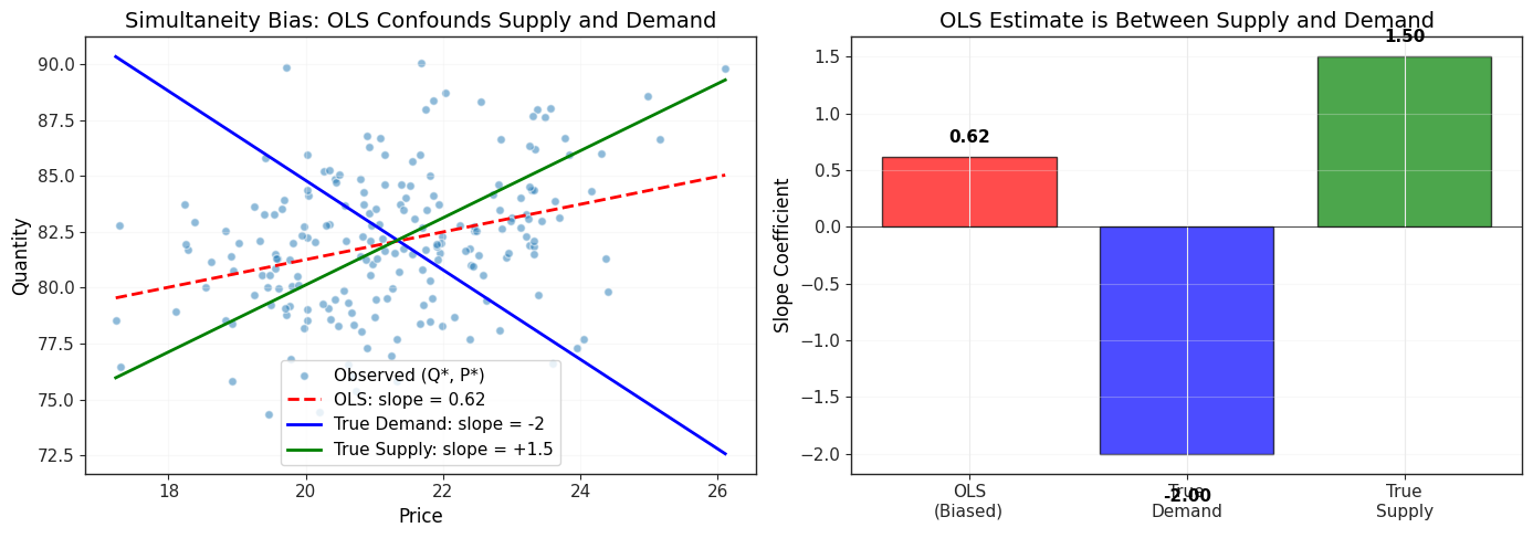
SIMULTANEITY BIAS DEMONSTRATION:
======================================================================
OLS slope:        0.6188
True demand slope: -2.0000
True supply slope:  1.5000

OLS is BIASED: It's between demand and supply, not equal to either!
OLS traces out the locus of equilibrium points, not a structural curve
16.3 Identifying and Estimating a Structural Equation¶
Before we can estimate a structural equation, we must determine if it is identified. Identification asks: “Can we uniquely recover the structural parameters from the reduced form?”
Identification Concepts¶
Three possible states:
Underidentified: Cannot recover structural parameters (not enough instruments)
Just identified: Can uniquely recover parameters (exactly identified)
Overidentified: More than enough instruments (can test overidentifying restrictions)
Order Condition for Identification¶
For equation in a system:
This is a necessary but not sufficient condition.
Rule of thumb: Each endogenous variable on the RHS needs at least one excluded exogenous variable (an exogenous variable that appears in other equations but not in this one) to serve as an instrument.
Rank Condition (Necessary and Sufficient)¶
The rank condition is more technical but guarantees identification. For equation :
The rank of the matrix of coefficients on variables excluded from equation must equal the number of endogenous variables in the system minus 1.
In practice:
Use order condition as a quick check
Order satisfied + economic theory -> likely identified
Formal rank condition checked by software
Example: Labor Supply and Wage Determination¶
Consider a woman’s labor supply decision:
Equation 1 (Labor Supply):
Equation 2 (Wage Equation):
Endogenous variables: hours, log(wage) Exogenous variables: educ, age, kidslt6, nwifeinc, exper, exper^2
Identification check for Equation 1:
Endogenous on RHS: log(wage) -> need 1 excluded exogenous variable
Excluded exogenous: exper, exper^2 -> have 2 instruments
Overidentified YES
Identification check for Equation 2:
Endogenous on RHS: hours -> need 1 excluded exogenous variable
Excluded exogenous: age, kidslt6, nwifeinc -> have 3 instruments
Overidentified YES
Example 16.5: Estimating the Mroz Labor-Supply System¶
We estimate the labor-supply equation by 2SLS, instrumenting log(wage) with exper and exper², which are excluded from the supply equation but enter the wage equation. The order condition delivers two excluded exogenous variables for one endogenous regressor, so the equation is overidentified, which means we can also run a Sargan-style overidentification test.
mroz = wool.data("mroz")
labor = mroz.dropna(subset=["lwage"]).copy()
labor["expersq"] = labor["exper"] ** 2

# OLS treats log(wage) as exogenous (biased under simultaneity).
ols_labor = smf.ols("hours ~ lwage + educ + age + kidslt6 + nwifeinc", data=labor).fit()

# 2SLS: instrument log(wage) with exper and exper^2.
iv_labor = IV2SLS.from_formula(
    "hours ~ 1 + educ + age + kidslt6 + nwifeinc + [lwage ~ exper + expersq]",
    data=labor,
).fit(cov_type="robust")

# First stage to confirm relevance.
first_stage = smf.ols(
    "lwage ~ exper + expersq + educ + age + kidslt6 + nwifeinc", data=labor,
).fit()
joint_F = first_stage.f_test("exper = 0, expersq = 0").fvalue

comparison = pd.DataFrame(
    {
        "OLS β̂": [ols_labor.params[k] for k in ["lwage", "educ", "kidslt6"]],
        "OLS SE": [ols_labor.bse[k] for k in ["lwage", "educ", "kidslt6"]],
        "2SLS β̂": [iv_labor.params[k] for k in ["lwage", "educ", "kidslt6"]],
        "2SLS SE": [iv_labor.std_errors[k] for k in ["lwage", "educ", "kidslt6"]],
    },
    index=["lwage (endogenous)", "educ", "kidslt6"],
)
display(comparison.round(2))
print(f"\nFirst-stage joint F on excluded instruments (exper, exper²): {float(joint_F):.2f}")
print(f"Sargan overid p-value (H₀: instruments valid): {iv_labor.sargan.pval:.3f}")
First-stage joint F on excluded instruments (exper, exper²): 9.33
Sargan overid p-value (H₀: instruments valid): 0.353
The OLS coefficient on lwage is near zero with a wide standard error; under simultaneity it does not consistently estimate the structural elasticity. The 2SLS coefficient is large and positive (women facing higher market wages work more hours, conditional on the controls), but the standard error is also enormous, and the first-stage F on the excluded instruments hovers near the conventional weak-instrument threshold of ten. This is what partial identification with weak instruments looks like in practice: the point estimate moves dramatically but the confidence interval is so wide that we cannot pin down the structural elasticity. The Sargan p-value does fail to reject the overidentifying restrictions, meaning the two excluded instruments are mutually consistent; mutual consistency, however, does not guarantee strength. The honest reading is that exper and exper² are not powerful enough instruments for lwage on this sample, and credible inference would require stronger excluded variables.
16.4 Systems with More Than Two Equations¶
When we have multiple equations, we can estimate them:
Equation-by-equation using 2SLS
Jointly using 3SLS (three-stage least squares)
Two-Stage Least Squares (2SLS) for Each Equation¶
Advantages:
Simple to implement (apply 2SLS to each equation separately)
Consistent estimators
Robust: if one equation is misspecified, others are unaffected
Disadvantages:
Ignores cross-equation error correlations
Less efficient than 3SLS when errors are correlated
Three-Stage Least Squares (3SLS)¶
3SLS is a system estimator that accounts for correlation between errors across equations.
Three stages:
First stage: Run reduced form regressions (like 2SLS first stage)
Second stage: Estimate each equation by 2SLS, save residuals
Third stage: Use residuals to estimate error covariance matrix, then apply generalized least squares (GLS) to the entire system
Advantages:
More efficient than 2SLS when errors are correlated across equations
System estimation can improve precision
Disadvantages:
If one equation is misspecified, all estimates are affected
More complex to implement
Requires correct specification of entire system
When to Use 3SLS vs 2SLS¶
Use 3SLS when:
You believe errors are correlated across equations
All equations are correctly specified
Want maximum efficiency
Use 2SLS when:
Uncertain about specification of some equations
Want robustness to misspecification
Simpler interpretation and diagnostics
Example 16.5: Labor Supply and Wage System¶
We’ll estimate the labor supply and wage system using both 2SLS and 3SLS.
# Load married women's labor force participation data
mroz = wool.data("mroz")

# Restrict to working women (non-missing wages)
mroz_working = mroz.dropna(subset=["lwage"])

print("SIMULTANEOUS EQUATIONS: Labor Supply and Wages")
print("=" * 70)
print("\nSample: Married women with observed wages")
print(f"Observations: {len(mroz_working)}")

print("\nSTRUCTURAL EQUATIONS:")
print("\n1. Labor Supply Equation:")
print(
    "   hours = beta_1_0 + beta_1_2*log(wage) + beta_1_1*educ + beta_1_2*age + beta_1_3*kidslt6 + beta_1_4*nwifeinc + u_1"
)
print("   Endogenous: log(wage)")
print("   Instruments: exper, exper^2")

print("\n2. Wage Equation:")
print("   log(wage) = beta_2_0 + beta_2_1*hours + beta_2_2*educ + beta_2_3*exper + beta_2_4*exper^2 + u_2")
print("   Endogenous: hours")
print("   Instruments: age, kidslt6, nwifeinc")

print("\nKEY QUESTION: Are hours and wages simultaneously determined?")
print("- Labor supply theory: Higher wages -> More hours worked (substitution effect)")
print("- Wage determination: More hours -> Lower hourly wage? (fatigue, bargaining)")

# Summary statistics
key_vars = ["hours", "lwage", "educ", "age", "kidslt6", "nwifeinc", "exper"]
display(mroz_working[key_vars].describe().round(2))
SIMULTANEOUS EQUATIONS: Labor Supply and Wages
======================================================================
Sample: Married women with observed wages
Observations: 428
STRUCTURAL EQUATIONS:
1. Labor Supply Equation:
hours = beta_1_0 + beta_1_2*log(wage) + beta_1_1*educ + beta_1_2*age + beta_1_3*kidslt6 + beta_1_4*nwifeinc + u_1
Endogenous: log(wage)
Instruments: exper, exper^2
2. Wage Equation:
log(wage) = beta_2_0 + beta_2_1*hours + beta_2_2*educ + beta_2_3*exper + beta_2_4*exper^2 + u_2
Endogenous: hours
Instruments: age, kidslt6, nwifeinc
KEY QUESTION: Are hours and wages simultaneously determined?
- Labor supply theory: Higher wages -> More hours worked (substitution effect)
- Wage determination: More hours -> Lower hourly wage? (fatigue, bargaining)
# EQUATION-BY-EQUATION 2SLS ESTIMATION
print("\n2SLS ESTIMATION (Equation-by-Equation)")
print("=" * 70)

# Equation 1: Labor Supply (hours depends on wage)
print("\nEQUATION 1: Labor Supply")
print("-" * 70)
print("Dependent variable: hours")
print("Endogenous regressor: log(wage)")
print("Instruments: exper, exper^2")

labor_supply_2sls = IV2SLS.from_formula(
    formula="hours ~ 1 + educ + age + kidslt6 + nwifeinc + "
    "[np.log(wage) ~ exper + I(exper**2)]",
    data=mroz_working,
).fit(cov_type="unadjusted", debiased=True)

table_supply = pd.DataFrame(
    {
        "Coefficient": labor_supply_2sls.params,
        "Std. Error": labor_supply_2sls.std_errors,
        "t-statistic": labor_supply_2sls.tstats,
        "p-value": labor_supply_2sls.pvalues,
    },
)
display(table_supply.round(4))

print(f"\nR-squared: {labor_supply_2sls.rsquared:.4f}")
print("First-stage F-stat: Check that instruments are relevant")
2SLS ESTIMATION (Equation-by-Equation)
======================================================================

EQUATION 1: Labor Supply
----------------------------------------------------------------------
Dependent variable: hours
Endogenous regressor: log(wage)
Instruments: exper, exper^2
R-squared: -2.0076
First-stage F-stat: Check that instruments are relevant
# Equation 2: Wage Equation (wage depends on hours)
print("\nEQUATION 2: Wage Equation")
print("-" * 70)
print("Dependent variable: log(wage)")
print("Endogenous regressor: hours")
print("Instruments: age, kidslt6, nwifeinc")

wage_eq_2sls = IV2SLS.from_formula(
    formula="np.log(wage) ~ 1 + educ + exper + I(exper**2) + "
    "[hours ~ age + kidslt6 + nwifeinc]",
    data=mroz_working,
).fit(cov_type="unadjusted", debiased=True)

table_wage = pd.DataFrame(
    {
        "Coefficient": wage_eq_2sls.params,
        "Std. Error": wage_eq_2sls.std_errors,
        "t-statistic": wage_eq_2sls.tstats,
        "p-value": wage_eq_2sls.pvalues,
    },
)
display(table_wage.round(4))

print(f"\nR-squared: {wage_eq_2sls.rsquared:.4f}")
EQUATION 2: Wage Equation
----------------------------------------------------------------------
Dependent variable: log(wage)
Endogenous regressor: hours
Instruments: age, kidslt6, nwifeinc
R-squared: 0.1257
# Check for cross-equation error correlation
print("\nCHECKING CROSS-EQUATION ERROR CORRELATION")
print("=" * 70)
print("If residuals are correlated, 3SLS will be more efficient than 2SLS")

# Get residuals from both equations
u1_hat = labor_supply_2sls.resids.values
u2_hat = wage_eq_2sls.resids.values

# Calculate correlation
cor_u1u2 = np.corrcoef(u1_hat, u2_hat)[0, 1]

print(f"\nCorrelation between residuals: {cor_u1u2:.4f}")

if abs(cor_u1u2) > 0.1:
    print(f"YES Substantial correlation (|{cor_u1u2:.4f}| > 0.1)")
    print("  -> 3SLS will be more efficient than 2SLS")
    print("  -> Errors across equations are related")
else:
    print(f"NO Low correlation (|{cor_u1u2:.4f}| <= 0.1)")
    print("  -> Little efficiency gain from 3SLS")
    print("  -> 2SLS and 3SLS will give similar results")
CHECKING CROSS-EQUATION ERROR CORRELATION
======================================================================
If residuals are correlated, 3SLS will be more efficient than 2SLS

Correlation between residuals: -0.9038
YES Substantial correlation (|-0.9038| > 0.1)
  -> 3SLS will be more efficient than 2SLS
  -> Errors across equations are related
# Interpretation of 2SLS results
print("\nINTERPRETATION OF 2SLS RESULTS")
print("=" * 70)

# Labor supply equation
wage_effect = labor_supply_2sls.params["np.log(wage)"]
wage_se = labor_supply_2sls.std_errors["np.log(wage)"]

print("\n1. LABOR SUPPLY EQUATION:")
print(f"   Effect of wage on hours: {wage_effect:.2f}")
if wage_effect > 0:
    print(f"   A 1% increase in wage -> {wage_effect:.2f} more hours worked per year")
    print("   YES Positive substitution effect (higher wage -> more labor supply)")
else:
    print(f"   A 1% increase in wage -> {abs(wage_effect):.2f} fewer hours worked")
    print("   YES Negative income effect dominates (higher wage -> less need to work)")

print(f"\n   Standard error: {wage_se:.4f}")
if abs(wage_effect / wage_se) > 1.96:
    print(f"   YES Statistically significant (t = {wage_effect / wage_se:.2f})")
else:
    print(f"   NO Not statistically significant (t = {wage_effect / wage_se:.2f})")

# Wage equation
hours_effect = wage_eq_2sls.params["hours"]
hours_se = wage_eq_2sls.std_errors["hours"]

print("\n2. WAGE EQUATION:")
print(f"   Effect of hours on log(wage): {hours_effect:.6f}")
if hours_effect > 0:
    print(f"   Each additional hour worked -> {100 * hours_effect:.4f}% higher wage")
    print("   Interpretation: Positive correlation (more productive workers work more)")
else:
    print(f"   Each additional hour worked -> {100 * abs(hours_effect):.4f}% lower wage")
    print("   Interpretation: Fatigue effect or part-time premium")

print(f"\n   Standard error: {hours_se:.6f}")
if abs(hours_effect / hours_se) > 1.96:
    print(f"   YES Statistically significant (t = {hours_effect / hours_se:.2f})")
else:
    print(f"   NO Not statistically significant (t = {hours_effect / hours_se:.2f})")
INTERPRETATION OF 2SLS RESULTS
======================================================================

1. LABOR SUPPLY EQUATION:
   Effect of wage on hours: 1639.56
   A 1% increase in wage -> 1639.56 more hours worked per year
   YES Positive substitution effect (higher wage -> more labor supply)

   Standard error: 470.5757
   YES Statistically significant (t = 3.48)

2. WAGE EQUATION:
   Effect of hours on log(wage): 0.000126
   Each additional hour worked -> 0.0126% higher wage
   Interpretation: Positive correlation (more productive workers work more)

   Standard error: 0.000255
   NO Not statistically significant (t = 0.49)
# THREE-STAGE LEAST SQUARES (3SLS)
print("\n\n3SLS ESTIMATION (System Estimation)")
print("=" * 70)
print("Estimates entire system jointly, accounting for cross-equation correlations")

# Define system of equations
system_formula = {
    "labor_supply": "hours ~ 1 + educ + age + kidslt6 + nwifeinc + "
    "[np.log(wage) ~ exper + I(exper**2)]",
    "wage_eq": "np.log(wage) ~ 1 + educ + exper + I(exper**2) + "
    "[hours ~ age + kidslt6 + nwifeinc]",
}

# Estimate system
system_3sls = IV3SLS.from_formula(system_formula, data=mroz_working)
results_3sls = system_3sls.fit(cov_type="unadjusted", debiased=True)

print("\n3SLS SYSTEM RESULTS")
print(results_3sls)
3SLS ESTIMATION (System Estimation)
======================================================================
Estimates entire system jointly, accounting for cross-equation correlations
3SLS SYSTEM RESULTS
                           System GLS Estimation Summary
===================================================================================
Estimator:                        GLS   Overall R-squared:                  -2.3957
No. Equations.:                     2   McElroy's R-squared:                 0.7846
No. Observations:                 428   Judge's (OLS) R-squared:            -2.3957
Date:                Thu, May 14 2026   Berndt's R-squared:                  0.5181
Time:                        00:16:04   Dhrymes's R-squared:                -2.3957
                                        Cov. Estimator:                  unadjusted
                                        Num. Constraints:                      None
               Equation: labor_supply, Dependent Variable: hours
================================================================================
              Parameter  Std. Err.     T-stat    P-value    Lower CI    Upper CI
--------------------------------------------------------------------------------
Intercept        2305.9     511.54     4.5077     0.0000      1300.4      3311.3
educ            -212.82     53.727    -3.9611     0.0001     -318.43     -107.21
age             -9.5150     7.9609    -1.1952     0.2327     -25.163      6.1331
kidslt6         -192.36     150.92    -1.2746     0.2032     -489.00      104.28
nwifeinc        -0.1770     3.5836    -0.0494     0.9606     -7.2210      6.8670
np.log(wage)     1781.9     439.88     4.0509     0.0001      917.30      2646.6

====================
    Instruments
--------------------
exper, I(exper ** 2)

               Equation: wage_eq, Dependent Variable: np.log(wage)
=================================================================================
               Parameter  Std. Err.     T-stat    P-value    Lower CI    Upper CI
---------------------------------------------------------------------------------
Intercept        -0.6939     0.3360    -2.0653     0.0395     -1.3543     -0.0335
educ              0.1127     0.0154     7.3355     0.0000      0.0825      0.1429
exper             0.0214     0.0154     1.3929     0.1644     -0.0088      0.0517
I(exper ** 2)    -0.0003     0.0003    -1.1303     0.2590     -0.0008      0.0002
hours             0.0002     0.0002     0.7707     0.4413     -0.0003      0.0007
======================
     Instruments
----------------------
age, kidslt6, nwifeinc
----------------------

Covariance Estimator:
Homoskedastic (Unadjusted) Covariance (Debiased: True, GLS: True)
# Compare 2SLS and 3SLS estimates
print("\n\nCOMPARISON: 2SLS vs 3SLS")
print("=" * 70)

print("\nLabor Supply Equation (hours):")
print("-" * 70)

comparison_supply = pd.DataFrame(
    {
        "2SLS": labor_supply_2sls.params,
        "2SLS SE": labor_supply_2sls.std_errors,
        "3SLS": results_3sls.params.filter(like="labor_supply"),
        "3SLS SE": results_3sls.std_errors.filter(like="labor_supply"),
    },
)

# Clean up index names for 3SLS
comparison_supply.index = [
    idx.replace("labor_supply_", "") for idx in comparison_supply.index
]
display(comparison_supply.round(4))

print("\nWage Equation (log(wage)):")
print("-" * 70)

comparison_wage = pd.DataFrame(
    {
        "2SLS": wage_eq_2sls.params,
        "2SLS SE": wage_eq_2sls.std_errors,
        "3SLS": results_3sls.params.filter(like="wage_eq"),
        "3SLS SE": results_3sls.std_errors.filter(like="wage_eq"),
    },
)

# Clean up index names for 3SLS
comparison_wage.index = [idx.replace("wage_eq_", "") for idx in comparison_wage.index]
display(comparison_wage.round(4))

print("\nKEY INSIGHTS:")
print("1. Coefficients: 2SLS and 3SLS estimates are similar (as expected)")
print("2. Standard Errors: 3SLS should have smaller SEs if errors are correlated")
print("3. Both methods account for simultaneity (unlike OLS which is biased)")
print("\nWHICH TO USE?")
print("- 3SLS: More efficient if system is correctly specified")
print("- 2SLS: More robust to misspecification of individual equations")
print("- In practice: Report both and compare for robustness")
COMPARISON: 2SLS vs 3SLS
======================================================================

Labor Supply Equation (hours):
----------------------------------------------------------------------
Wage Equation (log(wage)):
----------------------------------------------------------------------
KEY INSIGHTS:
1. Coefficients: 2SLS and 3SLS estimates are similar (as expected)
2. Standard Errors: 3SLS should have smaller SEs if errors are correlated
3. Both methods account for simultaneity (unlike OLS which is biased)

WHICH TO USE?
- 3SLS: More efficient if system is correctly specified
- 2SLS: More robust to misspecification of individual equations
- In practice: Report both and compare for robustness
16.5 Simultaneous Equations Models with Time Series¶
SEMs are particularly important for macroeconomic models where variables like GDP, consumption, investment, and interest rates are jointly determined.
Time Series Considerations¶
When applying SEMs to time series data:
Stationarity: Ensure variables are stationary (or cointegrated)
Serial correlation: Use robust standard errors or model dynamics explicitly
Lagged endogenous variables: Can serve as instruments (if predetermined)
Identification: Same rules apply, but more instruments available (lags)
Classic Macro SEM: IS-LM Model¶
A simplified Keynesian macro model:
IS Equation (Investment-Savings):
LM Equation (Liquidity-Money):
where:
= GDP (endogenous)
= interest rate (endogenous)
= government spending (exogenous)
= money supply (exogenous)
Identification:
IS equation: Excluded exogenous = -> identified
LM equation: Excluded exogenous = -> identified
Dynamic SEMs¶
In practice, macro models include dynamics (lags):
Lagged endogenous variables () are predetermined and can serve as instruments (assuming no serial correlation in errors).
# Conceptual example of macro SEM
print("TIME SERIES SEM: Macroeconomic Model")
print("=" * 70)

print("\nIS-LM MODEL (Conceptual)")
print("\nIS Equation (Goods Market Equilibrium):")
print("  Y = alpha_0 + alpha_1*r + alpha_2*G + u")
print("  Output (Y) depends negatively on interest rate (r)")
print("  Government spending (G) is exogenous policy variable")

print("\nLM Equation (Money Market Equilibrium):")
print("  r = beta_0 + beta_1*Y + beta_2*M + v")
print("  Interest rate (r) depends positively on output (Y)")
print("  Money supply (M) is exogenous policy variable")

print("\nIDENTIFICATION:")
print("YES IS equation: Use M (excluded from IS) as instrument for r")
print("YES LM equation: Use G (excluded from LM) as instrument for Y")

print("\nESTIMATION:")
print("- Apply 2SLS to each equation using appropriate instruments")
print("- Or use 3SLS for system estimation")
print("- With time series: Check stationarity, use robust SEs")

print("\nEXTENSIONS:")
print("- Add dynamics: Y_{t-1}, r_{t-1} as regressors")
print("- Use lags as instruments (if predetermined)")
print("- Model expectations: Forward-looking behavior")
TIME SERIES SEM: Macroeconomic Model
======================================================================
IS-LM MODEL (Conceptual)
IS Equation (Goods Market Equilibrium):
Y = alpha_0 + alpha_1*r + alpha_2*G + u
Output (Y) depends negatively on interest rate (r)
Government spending (G) is exogenous policy variable
LM Equation (Money Market Equilibrium):
r = beta_0 + beta_1*Y + beta_2*M + v
Interest rate (r) depends positively on output (Y)
Money supply (M) is exogenous policy variable
IDENTIFICATION:
YES IS equation: Use M (excluded from IS) as instrument for r
YES LM equation: Use G (excluded from LM) as instrument for Y
ESTIMATION:
- Apply 2SLS to each equation using appropriate instruments
- Or use 3SLS for system estimation
- With time series: Check stationarity, use robust SEs
EXTENSIONS:
- Add dynamics: Y_{t-1}, r_{t-1} as regressors
- Use lags as instruments (if predetermined)
- Model expectations: Forward-looking behavior
16.6 Simultaneous Equations Models with Panel Data¶
Panel data provides additional instruments through the time dimension, making identification easier. We can combine:
Fixed effects (control for unobserved heterogeneity)
Instrumental variables (address simultaneity)
Panel SEM Framework¶
Consider a two-equation panel system:
where:
= individual fixed effects
= exogenous variables
Instruments available:
Cross-sectional: Variables in other equations
Time-series: Lagged endogenous variables
Differences: First-differenced instruments
Estimation Approaches¶
Within-2SLS: Apply within transformation, then 2SLS
First-Difference 2SLS: First-difference, then 2SLS
System GMM: Use all available moment conditions
Example: Panel Data with Simultaneity¶
# Conceptual panel SEM example
print("PANEL DATA SEM: Firm Productivity and Training")
print("=" * 70)

print("\nSTRUCTURAL EQUATIONS:")

print("\n1. Productivity Equation:")
print("   log(output)_i_t = beta_1*training_i_t + controls + alpha_i + u_1_i_t")
print("   Productivity depends on training")

print("\n2. Training Decision:")
print("   training_i_t = beta_2*log(output)_i_t_-_1 + controls + c_i + u_2_i_t")
print("   Training depends on past productivity")

print("\nSIMULTANEITY:")
print("- Firms choose training based on productivity")
print("- Training affects future productivity")
print("- Need to account for both directions of causality")

print("\nIDENTIFICATION STRATEGY:")
print("YES Use lagged productivity as instrument for current training")
print("YES Use policy variables (grants) as instrument for training")
print("YES Fixed effects control for time-invariant firm heterogeneity")

print("\nESTIMATION:")
print("- First-difference to remove fixed effects")
print("- Apply 2SLS using lagged variables as instruments")
print("- Or use system GMM for efficiency")

print("\nADVANTAGES OF PANEL SEM:")
print("YES More instruments available (lags, differences)")
print("YES Control for unobserved heterogeneity (fixed effects)")
print("YES Richer identification from time variation")
print("YES Can test Granger causality")
PANEL DATA SEM: Firm Productivity and Training
======================================================================
STRUCTURAL EQUATIONS:
1. Productivity Equation:
log(output)_i_t = beta_1*training_i_t + controls + alpha_i + u_1_i_t
Productivity depends on training
2. Training Decision:
training_i_t = beta_2*log(output)_i_t_-_1 + controls + c_i + u_2_i_t
Training depends on past productivity
SIMULTANEITY:
- Firms choose training based on productivity
- Training affects future productivity
- Need to account for both directions of causality
IDENTIFICATION STRATEGY:
YES Use lagged productivity as instrument for current training
YES Use policy variables (grants) as instrument for training
YES Fixed effects control for time-invariant firm heterogeneity
ESTIMATION:
- First-difference to remove fixed effects
- Apply 2SLS using lagged variables as instruments
- Or use system GMM for efficiency
ADVANTAGES OF PANEL SEM:
YES More instruments available (lags, differences)
YES Control for unobserved heterogeneity (fixed effects)
YES Richer identification from time variation
YES Can test Granger causality
Key Considerations¶
Panel SEM challenges:
Weak instruments: Lagged variables may be weak instruments in short panels
Serial correlation: Errors may be serially correlated, invalidating some instruments
Dynamic panels: With lagged dependent variables, need GMM-type estimators
Unbalanced panels: Need to handle missing data carefully
Best practices:
Test for weak instruments (first-stage F-statistics)
Use robust/clustered standard errors
Test for serial correlation in errors
Consider system GMM for dynamic panels
Report both 2SLS and 3SLS for comparison
Chapter Summary¶
This chapter introduced simultaneous equations models for analyzing systems where multiple variables are jointly determined.
Key Concepts¶
Simultaneity:
Variables are mutually determined (endogenous)
OLS is biased and inconsistent
Need instrumental variables for identification
Structural vs. Reduced Form:
Structural: Economic relationships of interest
Reduced form: Endogenous variables as functions of exogenous only
Reduced form used to construct instruments
Identification:
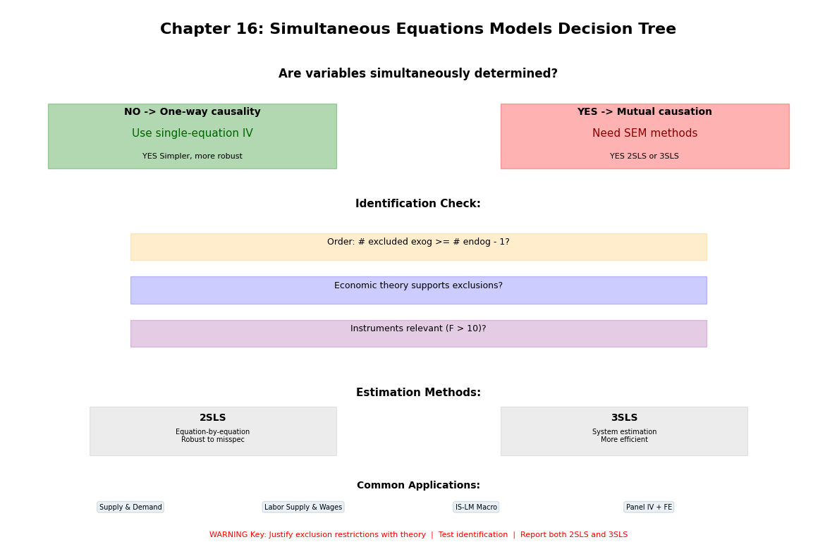
Order condition: # excluded exogenous >= # included endogenous - 1
Rank condition: More rigorous but checked by software
Need at least one excluded exogenous variable per endogenous RHS variable
Estimation Methods:
2SLS: Equation-by-equation, robust to misspecification
3SLS: System estimation, more efficient but less robust
Choice depends on confidence in full system specification
Extensions:
Time series: Macro models, IS-LM, lagged variables as instruments
Panel data: Fixed effects + IV, more instruments, GMM methods
When to Use SEMs¶
YES Use SEMs when:
Variables are clearly simultaneously determined
Have valid instruments (excluded exogenous variables)
Economic theory suggests mutual causation
NO Don’t use SEMs when:
One-way causality is plausible (use single-equation IV)
No valid instruments available
Can’t justify exclusion restrictions
Practical Recommendations¶
Start with 2SLS: More robust, easier to diagnose
Try 3SLS: If errors appear correlated across equations
Test identification: Check order and rank conditions
Test instruments: First-stage F-stats, overidentification tests
Robust SEs: Always use heteroskedasticity-robust or clustered SEs
Compare methods: Report both 2SLS and 3SLS for robustness
Remember: Simultaneous equations models require strong assumptions about identification. Carefully justify exclusion restrictions with economic theory!
Next Steps: Chapter 17 covers limited dependent variable models where the outcome is discrete, censored, or truncated.
Source
# Visual summary
fig, ax = plt.subplots(figsize=(12, 8))
ax.axis("off")

# Title
ax.text(
    0.5,
    0.95,
    "Chapter 16: Simultaneous Equations Models Decision Tree",
    ha="center",
    fontsize=16,
    fontweight="bold",
)

# Question 1: Simultaneity?
ax.text(
    0.5,
    0.87,
    "Are variables simultaneously determined?",
    ha="center",
    fontsize=12,
    fontweight="bold",
)

# Branch: No
ax.add_patch(
    plt.Rectangle((0.05, 0.70), 0.35, 0.12, fill=True, alpha=0.3, color="green")
)
ax.text(
    0.225, 0.80, "NO -> One-way causality", ha="center", fontsize=10, fontweight="bold"
)
ax.text(
    0.225, 0.76, "Use single-equation IV", ha="center", fontsize=11, color="darkgreen"
)
ax.text(0.225, 0.72, "YES Simpler, more robust", ha="center", fontsize=8)

# Branch: Yes
ax.add_patch(plt.Rectangle((0.6, 0.70), 0.35, 0.12, fill=True, alpha=0.3, color="red"))
ax.text(
    0.775, 0.80, "YES -> Mutual causation", ha="center", fontsize=10, fontweight="bold"
)
ax.text(0.775, 0.76, "Need SEM methods", ha="center", fontsize=11, color="darkred")
ax.text(0.775, 0.72, "YES 2SLS or 3SLS", ha="center", fontsize=8)

# Identification
ax.text(0.5, 0.63, "Identification Check:", ha="center", fontsize=11, fontweight="bold")

checks = [
    "Order: # excluded exog >= # endog - 1?",
    "Economic theory supports exclusions?",
    "Instruments relevant (F > 10)?",
]
colors_check = ["orange", "blue", "purple"]
for i, (check, color) in enumerate(zip(checks, colors_check, strict=False)):
    y_pos = 0.56 - i * 0.08
    ax.add_patch(
        plt.Rectangle(
            (0.15, y_pos - 0.03), 0.7, 0.05, fill=True, alpha=0.2, color=color
        )
    )
    ax.text(0.5, y_pos, check, ha="center", fontsize=9)

# Estimation methods
ax.text(0.5, 0.28, "Estimation Methods:", ha="center", fontsize=11, fontweight="bold")

methods = [
    ("2SLS", "Equation-by-equation\nRobust to misspec"),
    ("3SLS", "System estimation\nMore efficient"),
]

for i, (method, desc) in enumerate(methods):
    x_pos = 0.25 if i == 0 else 0.75
    ax.add_patch(
        plt.Rectangle(
            (x_pos - 0.15, 0.17), 0.3, 0.09, fill=True, alpha=0.15, color="gray"
        )
    )
    ax.text(x_pos, 0.235, method, ha="center", fontsize=10, fontweight="bold")
    ax.text(x_pos, 0.195, desc, ha="center", fontsize=7)

# Applications
ax.text(0.5, 0.11, "Common Applications:", ha="center", fontsize=10, fontweight="bold")

apps = ["Supply & Demand", "Labor Supply & Wages", "IS-LM Macro", "Panel IV + FE"]
for i, app in enumerate(apps):
    x_pos = 0.15 + i * 0.21
    ax.text(
        x_pos,
        0.07,
        app,
        ha="center",
        fontsize=7,
        bbox=dict(boxstyle="round", alpha=0.1),
    )

# Bottom warnings
ax.text(
    0.5,
    0.02,
    "WARNING Key: Justify exclusion restrictions with theory  |  Test identification  |  Report both 2SLS and 3SLS",
    ha="center",
    fontsize=8,
    color="red",
)

plt.tight_layout()
plt.show()