14. Advanced Panel Data Methods

Learning Objectives

TODO: Add learning objectives for this chapter. The sections below provide a starting template:

14.1 TODO: objective for “Fixed Effects Estimation”

14.2 TODO: objective for “Random Effects Estimation”

14.3 TODO: objective for “The Correlated Random Effects Approach”

14.4 TODO: objective for “General Policy Analysis with Panel Data”

14.5 TODO: objective for “Applying Panel Data Methods to Other Data Structures”

Advanced panel data methods provide researchers with powerful tools for addressing endogeneity arising from time-invariant unobserved heterogeneity. This chapter develops the fixed effects (FE) and random effects (RE) estimators, establishing the theoretical foundations, computational procedures, and inferential frameworks that make these approaches central to modern applied econometric analysis.

The development proceeds systematically through the panel data toolkit. We establish the fixed effects estimator as the within transformation that eliminates individual-specific effects (Section 14.1), introduce the random effects estimator under the assumption that individual effects are uncorrelated with regressors (Section 14.2), develop the Hausman test for choosing between FE and RE specifications along with correlated random effects approaches that bridge the two methods (Section 14.3), examine robust inference procedures including clustered standard errors for panel data (Section 14.4), and extend these methods to unbalanced panels, repeated cross sections, and policy evaluation contexts (Section 14.5). Throughout, we implement estimators using Python’s linearmodels package and demonstrate applications to labor economics, health economics, and development studies.

# Import required libraries
import matplotlib.pyplot as plt
import pandas as pd
import statsmodels.formula.api as smf
import wooldridge as wool
from IPython.display import display
from linearmodels import PanelOLS, RandomEffects

plt.style.use("theme.mplstyle")

14.1 Fixed Effects Estimation¶

The fixed effects (FE) estimator, also called the within estimator, removes the unobserved individual effect $a_i$ by de-meaning all variables. This is one of the most widely used panel data estimators in economics.

The Fixed Effects Model¶

Consider the standard panel data model with unobserved heterogeneity:

y_{it} = \beta_1 x_{1,it} + \beta_2 x_{2,it} + \ldots + \beta_k x_{k,it} + a_i + u_{it}

(1)

where:

$a_i$ = individual-specific unobserved effect (time-invariant)
$u_{it}$ = idiosyncratic error (varies over $i$ and $t$ )
The key problem: $a_i$ may be correlated with the $x$ variables

The Within Transformation¶

The FE estimator eliminates $a_i$ by subtracting the individual-specific time average from each variable:

\ddot{y}_{it} = y_{it} - \bar{y}_i = \beta_1 \ddot{x}_{1,it} + \ldots + \beta_k \ddot{x}_{k,it} + \ddot{u}_{it}

(2)

where $\bar{y}_i = T_i^{-1} \sum_{t=1}^{T_i} y_{it}$ is the time average for individual $i$ , and $\ddot{y}_{it} = y_{it} - \bar{y}_i$ is the de-meaned (or “within”) transformation.

Notice that $a_i$ has disappeared because $a_i - a_i = 0$ !

Properties of the FE Estimator¶

Consistency: FE is consistent even if $a_i$ is correlated with the $x$ variables
Strict exogeneity required: $E(u_{it}|x_{i1}, \ldots, x_{iT}, a_i) = 0$ for all $t$
Time-invariant variables: Cannot estimate effects of variables that don’t change over time
Standard errors: Should be clustered at the individual level to account for serial correlation

Example 14.1: Effect of Job Training on Firm Productivity¶

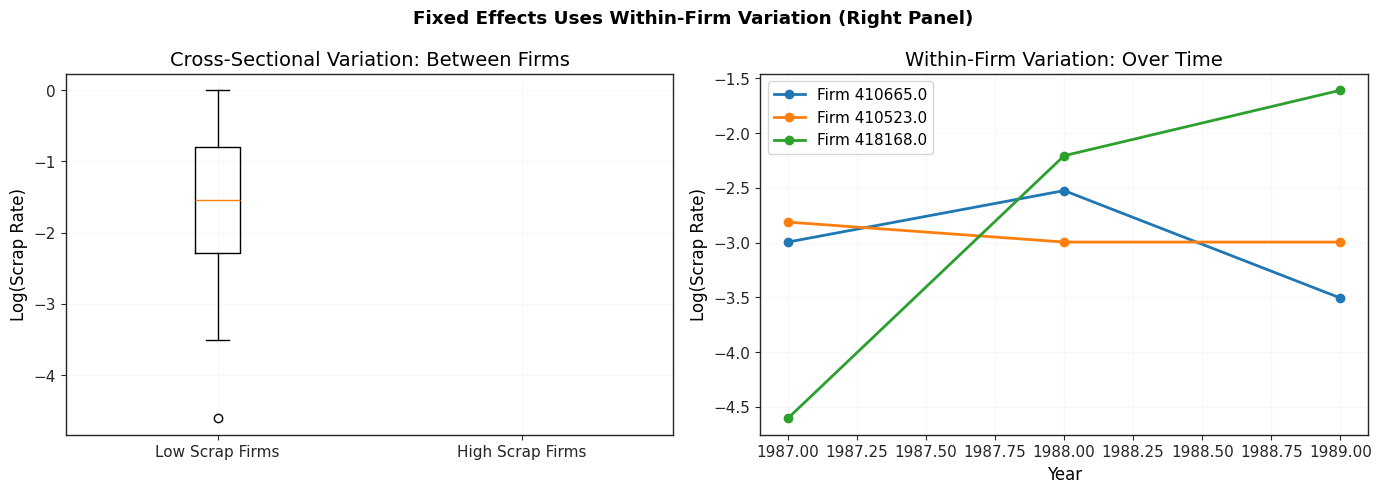
We’ll analyze whether job training grants improve firm productivity using data on manufacturing firms. The outcome is the (log) scrap rate, and we control for unobserved firm characteristics that might affect both training and productivity.

# Load job training panel data
jtrain = wool.data("jtrain")

print("Dataset Information:")
print(f"Total observations: {len(jtrain)}")
print(f"Number of firms: {jtrain['fcode'].nunique()}")
print(f"Years: {sorted(jtrain['year'].unique())}")
print(f"Time periods per firm: {len(jtrain['year'].unique())}")

# Display variable descriptions
print("\nKey Variables:")
print("- lscrap: log(scrap rate) - our outcome variable")
print("- d88, d89: year dummies for 1988 and 1989")
print("- grant: =1 if firm received grant this year")
print("- grant_1: =1 if firm received grant last year")
print("- fcode: firm identifier")

# Show first observations for a few firms
display(jtrain.head(15))

Dataset Information:
Total observations: 471
Number of firms: 157
Years: [np.int64(1987), np.int64(1988), np.int64(1989)]
Time periods per firm: 3

Key Variables:
- lscrap: log(scrap rate) - our outcome variable
- d88, d89: year dummies for 1988 and 1989
- grant: =1 if firm received grant this year
- grant_1: =1 if firm received grant last year
- fcode: firm identifier

# Summary statistics
key_vars = ["lscrap", "grant", "grant_1", "d88", "d89"]
print("Summary Statistics:")
display(jtrain[key_vars].describe().round(4))

Summary Statistics:

Manual Fixed Effects Estimation¶

To understand FE intuitively, let’s first estimate it manually by de-meaning the variables:

# Set up panel structure
jtrain_panel = jtrain.copy()
jtrain_panel["entity"] = jtrain_panel["fcode"]
jtrain_panel = jtrain_panel.set_index(["fcode", "year"])

# Manual computation: subtract entity (firm) means from each variable
# The suffix '_w' denotes "within" (de-meaned) variables
jtrain_panel["lscrap_w"] = jtrain_panel["lscrap"] - jtrain_panel.groupby("fcode")[
    "lscrap"
].transform("mean")
jtrain_panel["d88_w"] = jtrain_panel["d88"] - jtrain_panel.groupby("fcode")[
    "d88"
].transform("mean")
jtrain_panel["d89_w"] = jtrain_panel["d89"] - jtrain_panel.groupby("fcode")[
    "d89"
].transform("mean")
jtrain_panel["grant_w"] = jtrain_panel["grant"] - jtrain_panel.groupby("fcode")[
    "grant"
].transform("mean")
jtrain_panel["grant_1_w"] = jtrain_panel["grant_1"] - jtrain_panel.groupby("fcode")[
    "grant_1"
].transform("mean")

print("Manual de-meaning completed")
print("\nExample: First firm's de-meaned values")
first_firm = jtrain_panel.index.get_level_values(0).unique()[0]
display(jtrain_panel.loc[first_firm, ["lscrap", "lscrap_w", "grant", "grant_w"]])

Manual de-meaning completed

Example: First firm's de-meaned values

# Estimate FE model manually using OLS on de-meaned data
# Note: no intercept (0 +) because de-meaned data has mean zero
model_manual = smf.ols(
    formula="lscrap_w ~ 0 + d88_w + d89_w + grant_w + grant_1_w",
    data=jtrain_panel,
)
results_manual = model_manual.fit()

print("MANUAL FIXED EFFECTS ESTIMATION")
print("=" * 70)
print("(Estimated using OLS on de-meaned variables)")
print()

table_manual = pd.DataFrame(
    {
        "Coefficient": results_manual.params,
        "Std. Error": results_manual.bse,
        "t-statistic": results_manual.tvalues,
        "p-value": results_manual.pvalues,
    },
)
display(table_manual.round(4))
print(f"\nR-squared (within): {results_manual.rsquared:.4f}")
print(f"Observations: {int(results_manual.nobs)}")

MANUAL FIXED EFFECTS ESTIMATION
======================================================================
(Estimated using OLS on de-meaned variables)


R-squared (within): 0.2010
Observations: 162

Automatic Fixed Effects Estimation¶

Now let’s use the specialized PanelOLS estimator with EntityEffects, which handles everything automatically:

# Automatic FE estimation using linearmodels
# EntityEffects automatically includes individual fixed effects
# TimeEffects automatically includes time fixed effects
model_auto = PanelOLS.from_formula(
    formula="lscrap ~ d88 + d89 + grant + grant_1 + EntityEffects",
    data=jtrain_panel,
)
results_auto = model_auto.fit(cov_type="clustered", cluster_entity=True)

print("\nAUTOMATIC FIXED EFFECTS ESTIMATION")
print("=" * 70)
print("(Using PanelOLS with EntityEffects and clustered SEs)")
print()

table_auto = pd.DataFrame(
    {
        "Coefficient": results_auto.params,
        "Std. Error": results_auto.std_errors,
        "t-statistic": results_auto.tstats,
        "p-value": results_auto.pvalues,
    },
)
display(table_auto.round(4))
print(f"\nR-squared (within): {results_auto.rsquared_within:.4f}")
print(f"R-squared (overall): {results_auto.rsquared_overall:.4f}")
print(f"Observations: {results_auto.nobs}")
print(f"Entities (firms): {results_auto.entity_info['total']}")


AUTOMATIC FIXED EFFECTS ESTIMATION
======================================================================
(Using PanelOLS with EntityEffects and clustered SEs)

/home/runner/work/merino/merino/.venv/lib/python3.11/site-packages/linearmodels/panel/model.py:1258: MissingValueWarning: 
Inputs contain missing values. Dropping rows with missing observations.
  super().__init__(dependent, exog, weights=weights, check_rank=check_rank)


R-squared (within): 0.2010
R-squared (overall): -0.0839
Observations: 162
Entities (firms): 54.0

# Compare manual and automatic estimates
print("\nCOMPARISON: Manual vs Automatic FE Estimates")
print("=" * 70)

comparison = pd.DataFrame(
    {
        "Manual FE": results_manual.params,
        "Automatic FE": results_auto.params,
        "Difference": results_manual.params - results_auto.params,
    },
)
display(comparison.round(6))

print("\nNote: Coefficients are identical (differences due to rounding).")
print("Standard errors differ because automatic FE uses clustered SEs.")


COMPARISON: Manual vs Automatic FE Estimates
======================================================================


Note: Coefficients are identical (differences due to rounding).
Standard errors differ because automatic FE uses clustered SEs.

# Interpretation of results
print("\nINTERPRETATION OF FIXED EFFECTS ESTIMATES:")
print("=" * 70)

grant_coef = results_auto.params["grant"]
grant_se = results_auto.std_errors["grant"]
grant_1_coef = results_auto.params["grant_1"]

print(f"\n1. Current Year Grant Effect: {grant_coef:.4f}")
if abs(grant_coef / grant_se) < 1.96:
    print(
        "   The grant has NO statistically significant effect on scrap rates this year",
    )
    print(
        f"   (t-stat = {grant_coef / grant_se:.2f}, p-value = {results_auto.pvalues['grant']:.3f})"
    )
else:
    print(
        f"   The grant {'reduces' if grant_coef < 0 else 'increases'} log(scrap) by {abs(grant_coef):.4f}",
    )
    print(
        f"   This is approximately a {100 * abs(grant_coef):.2f}% change in scrap rates"
    )

print(f"\n2. Lagged Grant Effect (grant_1): {grant_1_coef:.4f}")
print(
    f"   Receiving a grant LAST year {'reduces' if grant_1_coef < 0 else 'increases'} log(scrap) by {abs(grant_1_coef):.4f}",
)
print(
    f"   This is approximately a {100 * abs(grant_1_coef):.2f}% change in scrap rates"
)
print("   (The effect may take time to materialize as workers apply new skills)")

print("\n3. Firm Fixed Effects:")
print("   The model controls for all time-invariant firm characteristics:")
print("   - Management quality")
print("   - Firm culture and organization")
print("   - Geographic location")
print("   - Industry-specific factors")
print("   - Any other unobserved factors that don't change over time")


INTERPRETATION OF FIXED EFFECTS ESTIMATES:
======================================================================

1. Current Year Grant Effect: -0.2523
   The grant has NO statistically significant effect on scrap rates this year
   (t-stat = -1.78, p-value = 0.079)

2. Lagged Grant Effect (grant_1): -0.4216
   Receiving a grant LAST year reduces log(scrap) by 0.4216
   This is approximately a 42.16% change in scrap rates
   (The effect may take time to materialize as workers apply new skills)

3. Firm Fixed Effects:
   The model controls for all time-invariant firm characteristics:
   - Management quality
   - Firm culture and organization
   - Geographic location
   - Industry-specific factors
   - Any other unobserved factors that don't change over time

Visualizing the Fixed Effects¶

# Visualize variation in scrap rates across firms and over time
fig, axes = plt.subplots(1, 2, figsize=(14, 5))

# Panel A: Variation across firms (box plots)
firm_means = jtrain.groupby("fcode")["lscrap"].mean().sort_values()
top_10_firms = firm_means.head(10).index
bottom_10_firms = firm_means.tail(10).index
selected_firms = list(top_10_firms) + list(bottom_10_firms)

jtrain_selected = jtrain[jtrain["fcode"].isin(selected_firms)]
jtrain_selected["firm_category"] = jtrain_selected["fcode"].apply(
    lambda x: "Low scrap" if x in top_10_firms else "High scrap",
)

axes[0].boxplot(
    [
        jtrain_selected[jtrain_selected["firm_category"] == "Low scrap"]["lscrap"],
        jtrain_selected[jtrain_selected["firm_category"] == "High scrap"]["lscrap"],
    ],
    labels=["Low Scrap Firms", "High Scrap Firms"],
)
axes[0].set_ylabel("Log(Scrap Rate)")
axes[0].set_title("Cross-Sectional Variation: Between Firms")
axes[0].grid(True, alpha=0.3)

# Panel B: Within-firm variation over time (selected firms)
for firm in list(top_10_firms)[:3]:
    firm_data = jtrain[jtrain["fcode"] == firm].sort_values("year")
    axes[1].plot(
        firm_data["year"], firm_data["lscrap"], marker="o", label=f"Firm {firm}"
    )

axes[1].set_xlabel("Year")
axes[1].set_ylabel("Log(Scrap Rate)")
axes[1].set_title("Within-Firm Variation: Over Time")
axes[1].legend()
axes[1].grid(True, alpha=0.3)

plt.suptitle(
    "Fixed Effects Uses Within-Firm Variation (Right Panel)", fontweight="bold"
)
plt.tight_layout()
plt.show()

/tmp/ipykernel_2813/3398153719.py:15: MatplotlibDeprecationWarning: The 'labels' parameter of boxplot() has been renamed 'tick_labels' since Matplotlib 3.9; support for the old name will be dropped in 3.11.
  axes[0].boxplot(

14.2 Random Effects Estimation¶

The random effects (RE) estimator is a generalized least squares (GLS) estimator that can be more efficient than FE when the unobserved effect is uncorrelated with the explanatory variables.

The Random Effects Model¶

The RE model assumes:

y_{it} = \beta_0 + \beta_1 x_{1,it} + \ldots + \beta_k x_{k,it} + a_i + u_{it}

(3)

Key RE assumption: $E(a_i | x_{i1}, \ldots, x_{iT}) = \beta_0$

This means $a_i$ is uncorrelated with all $x$ variables. This is a strong assumption!

Why Random Effects?¶

Efficiency: If the RE assumption holds, RE is more efficient than FE Time-invariant variables: RE can estimate effects of variables that don’t vary over time Between variation: RE uses both within and between variation

The RE Transformation¶

RE uses a quasi-demeaning transformation:

y_{it} - \theta \bar{y}_i = \beta_0(1-\theta) + \beta_1(x_{1,it} - \theta \bar{x}_{1,i}) + \ldots + v_{it}

(4)

where:

$\theta = 1 - \sqrt{\sigma_u^2 / (\sigma_u^2 + T\sigma_a^2)}$
$\theta \in [0, 1]$ depending on the relative importance of $a_i$ vs $u_{it}$
If $\theta = 1$ : RE reduces to FE (full de-meaning)
If $\theta = 0$ : RE reduces to pooled OLS (no de-meaning)

Example 14.2: Wage Equation with Time-Varying Education Returns¶

We’ll estimate the returns to education, marriage, and union membership using a panel of male workers.

# Load wage panel data
wagepan = wool.data("wagepan")

print("Dataset Information:")
print(f"Total observations: {len(wagepan)}")
print(f"Number of individuals: {wagepan['nr'].nunique()}")
print(f"Years: {sorted(wagepan['year'].unique())}")
print(f"Observations per person: {len(wagepan) / wagepan['nr'].nunique():.1f}")

print("\nKey Variables:")
print("- lwage: log(wage)")
print("- educ: years of education (time-invariant for most)")
print("- married: =1 if married")
print("- union: =1 if union member")
print("- nr: person identifier")

display(wagepan.head(12))

Dataset Information:
Total observations: 4360
Number of individuals: 545
Years: [np.int64(1980), np.int64(1981), np.int64(1982), np.int64(1983), np.int64(1984), np.int64(1985), np.int64(1986), np.int64(1987)]
Observations per person: 8.0

Key Variables:
- lwage: log(wage)
- educ: years of education (time-invariant for most)
- married: =1 if married
- union: =1 if union member
- nr: person identifier

# Set up panel structure
wagepan_panel = wagepan.set_index(["nr", "year"], drop=False)

# Summary statistics
print("Summary Statistics:")
display(wagepan[["lwage", "educ", "married", "union", "exper"]].describe().round(3))

Summary Statistics:

We want to allow education returns to vary by year (perhaps due to skill-biased technological change):

# Fixed Effects model with time-varying education returns
# C(year)*educ creates interactions between year dummies and education
# year is already a column since we used drop=False in set_index
fe_model = PanelOLS.from_formula(
    formula="lwage ~ married + union + C(year)*educ + EntityEffects",
    data=wagepan_panel,
    drop_absorbed=True,  # Don't show individual dummies
)
fe_results = fe_model.fit(cov_type="clustered", cluster_entity=True)

print("FIXED EFFECTS ESTIMATION: Time-Varying Returns to Education")
print("=" * 70)

fe_table = pd.DataFrame(
    {
        "Coefficient": fe_results.params,
        "Std. Error": fe_results.std_errors,
        "t-statistic": fe_results.tstats,
        "p-value": fe_results.pvalues,
    },
)
display(fe_table.round(4))
print(f"\nR-squared (within): {fe_results.rsquared_within:.4f}")
print(f"Observations: {fe_results.nobs}")

FIXED EFFECTS ESTIMATION: Time-Varying Returns to Education
======================================================================

/tmp/ipykernel_2813/264589140.py:9: AbsorbingEffectWarning: 
Variables have been fully absorbed and have removed from the regression:

educ

  fe_results = fe_model.fit(cov_type="clustered", cluster_entity=True)


R-squared (within): 0.1708
Observations: 4360

# Interpretation
print("\nINTERPRETATION OF FE RESULTS:")
print("=" * 70)

married_coef = fe_results.params["married"]
union_coef = fe_results.params["union"]

print(f"\n1. Marriage Premium: {married_coef:.4f}")
print(f"   Being married increases log(wage) by {married_coef:.4f}")
print(f"   Approximately {100 * married_coef:.2f}% higher wages for married men")

print(f"\n2. Union Premium: {union_coef:.4f}")
print(f"   Union membership increases log(wage) by {union_coef:.4f}")
print(f"   Approximately {100 * union_coef:.2f}% higher wages for union members")

print("\n3. Education Returns by Year:")
print("   Base year return captured by year fixed effects")
print("   Interaction terms show how returns changed over time")

# Extract education*year interactions
educ_interactions = {
    k: v for k, v in fe_results.params.items() if "educ" in k and ":" in k
}
if educ_interactions:
    print("\n   Year-specific changes in education returns:")
    for term, coef in educ_interactions.items():
        print(f"   {term}: {coef:.4f}")


INTERPRETATION OF FE RESULTS:
======================================================================

1. Marriage Premium: 0.0548
   Being married increases log(wage) by 0.0548
   Approximately 5.48% higher wages for married men

2. Union Premium: 0.0830
   Union membership increases log(wage) by 0.0830
   Approximately 8.30% higher wages for union members

3. Education Returns by Year:
   Base year return captured by year fixed effects
   Interaction terms show how returns changed over time

   Year-specific changes in education returns:
   C(year)[T.1981]:educ: 0.0116
   C(year)[T.1982]:educ: 0.0148
   C(year)[T.1983]:educ: 0.0171
   C(year)[T.1984]:educ: 0.0166
   C(year)[T.1985]:educ: 0.0237
   C(year)[T.1986]:educ: 0.0274
   C(year)[T.1987]:educ: 0.0304

14.3 The Correlated Random Effects Approach¶

The Correlated Random Effects (CRE) approach, developed by Chamberlain (1982) and Mundlak (1978), provides a middle ground between FE and RE. It allows correlation between $a_i$ and the $x$ variables in a flexible way.

The CRE Specification¶

The key idea: model the correlation between $a_i$ and $x_{it}$ explicitly:

a_i = \psi_0 + \psi_1 \bar{x}_{1,i} + \psi_2 \bar{x}_{2,i} + \ldots + \psi_k \bar{x}_{k,i} + r_i

(5)

where $\bar{x}_{j,i} = T_i^{-1} \sum_{t=1}^{T_i} x_{j,it}$ is the time average of variable $j$ for individual $i$ .

Substituting into the original model:

y_{it} = \beta_0 + \beta_1 x_{1,it} + \ldots + \beta_k x_{k,it} + \psi_1 \bar{x}_{1,i} + \ldots + \psi_k \bar{x}_{k,i} + r_i + u_{it}

(6)

Now $r_i$ is uncorrelated with all $x$ variables (by construction), so we can use RE methods!

Interpretation of CRE Coefficients¶

$\beta_j$ = within effect (same as FE estimate)
$\beta_j + \psi_j$ = overall effect including between variation
$\psi_j$ = difference between overall and within effects
If $\psi_j = 0$ : no correlation between $a_i$ and $x_j$ (RE assumption holds)

Example: CRE Wage Equation¶

Let’s estimate the wage equation using CRE to test whether marriage and union status are correlated with unobserved ability ( $a_i$ ):

# Prepare data for CRE
wagepan_cre = wagepan.copy()
wagepan_cre["t"] = wagepan_cre["year"]
wagepan_cre["entity"] = wagepan_cre["nr"]

# Create time-averages (group means) for time-varying variables
# The suffix '_b' denotes "between" (time average)
wagepan_cre["married_b"] = wagepan_cre.groupby("nr")["married"].transform("mean")
wagepan_cre["union_b"] = wagepan_cre.groupby("nr")["union"].transform("mean")

# Set panel index, keeping year as column for formulas
wagepan_cre = wagepan_cre.set_index(["nr", "year"], drop=False)

print("Created time-averaged variables:")
print("married_b: time average of married status for each person")
print("union_b: time average of union status for each person")
print("\nFirst few observations:")
display(wagepan_cre[["lwage", "married", "married_b", "union", "union_b"]].head(12))

Created time-averaged variables:
married_b: time average of married status for each person
union_b: time average of union status for each person

First few observations:

# Estimate CRE model using Random Effects
# Include both the original variables AND their time averages
cre_model = RandomEffects.from_formula(
    formula="lwage ~ married + union + educ + black + hisp + married_b + union_b",
    data=wagepan_cre,
)
cre_results = cre_model.fit(cov_type="clustered", cluster_entity=True)

print("CORRELATED RANDOM EFFECTS ESTIMATION")
print("=" * 70)

cre_table = pd.DataFrame(
    {
        "Coefficient": cre_results.params,
        "Std. Error": cre_results.std_errors,
        "t-statistic": cre_results.tstats,
        "p-value": cre_results.pvalues,
    },
)
display(cre_table.round(4))
print(f"\nObservations: {cre_results.nobs}")

CORRELATED RANDOM EFFECTS ESTIMATION
======================================================================


Observations: 4360

# Interpretation and hypothesis testing
print("\nINTERPRETATION OF CRE RESULTS:")
print("=" * 70)

# Within effects (same as FE)
married_within = cre_results.params["married"]
union_within = cre_results.params["union"]

# Between effects (time-averaged variables)
married_between = cre_results.params["married_b"]
union_between = cre_results.params["union_b"]

print("\n1. WITHIN EFFECTS (changes over time):")
print(f"   married: {married_within:.4f}")
print(f"   Getting married increases wages by {100 * married_within:.2f}%")
print(f"\n   union: {union_within:.4f}")
print(f"   Joining a union increases wages by {100 * union_within:.2f}%")

print("\n2. BETWEEN EFFECTS (time-averaged):")
print(f"   married_b: {married_between:.4f}")
if abs(married_between / cre_results.std_errors["married_b"]) > 1.96:
    print(
        "   Men who are married more often have "
        f"{'higher' if married_between > 0 else 'lower'} unobserved ability"
    )
    print("   (statistically significant at 5% level)")
else:
    print("   No significant correlation with unobserved ability")

print(f"\n   union_b: {union_between:.4f}")
if abs(union_between / cre_results.std_errors["union_b"]) > 1.96:
    print(
        "   Men who are union members more often have "
        f"{'higher' if union_between > 0 else 'lower'} unobserved ability"
    )
    print("   (statistically significant at 5% level)")
else:
    print("   No significant correlation with unobserved ability")

print("\n3. TIME-INVARIANT VARIABLES:")
educ_coef = cre_results.params["educ"]
print(f"   educ: {educ_coef:.4f}")
print(f"   One additional year of education increases wages by {100 * educ_coef:.2f}%")
print("   (Cannot be estimated with FE because education doesn't vary)")

print("\n4. TESTING THE RANDOM EFFECTS ASSUMPTION:")
print("   Null hypothesis: married_b = union_b = 0")
print("   (i.e., no correlation between time-averages and unobserved effect)")
if (
    abs(married_between / cre_results.std_errors["married_b"]) > 1.96
    or abs(union_between / cre_results.std_errors["union_b"]) > 1.96
):
    print("   REJECT: At least one time-average is significant")
    print("   -> Standard RE assumption is violated")
    print("   -> Should use FE or CRE instead of plain RE")
else:
    print("   FAIL TO REJECT: Time-averages not significant")
    print("   -> Standard RE assumption is plausible")
    print("   -> Can use plain RE for efficiency")


INTERPRETATION OF CRE RESULTS:
======================================================================

1. WITHIN EFFECTS (changes over time):
   married: 0.2417
   Getting married increases wages by 24.17%

   union: 0.0700
   Joining a union increases wages by 7.00%

2. BETWEEN EFFECTS (time-averaged):
   married_b: -0.0436
   No significant correlation with unobserved ability

   union_b: 0.2105
   Men who are union members more often have higher unobserved ability
   (statistically significant at 5% level)

3. TIME-INVARIANT VARIABLES:
   educ: 0.1257
   One additional year of education increases wages by 12.57%
   (Cannot be estimated with FE because education doesn't vary)

4. TESTING THE RANDOM EFFECTS ASSUMPTION:
   Null hypothesis: married_b = union_b = 0
   (i.e., no correlation between time-averages and unobserved effect)
   REJECT: At least one time-average is significant
   -> Standard RE assumption is violated
   -> Should use FE or CRE instead of plain RE

Hausman Test: FE vs RE¶

The Hausman test compares FE and RE estimates to test whether the RE assumption holds:

# For demonstration: estimate plain RE (without time averages)
re_model = RandomEffects.from_formula(
    formula="lwage ~ married + union + educ + black + hisp",
    data=wagepan_cre,
)
re_results = re_model.fit(cov_type="clustered", cluster_entity=True)

print("PLAIN RANDOM EFFECTS (for comparison)")
print("=" * 70)
re_table = pd.DataFrame(
    {
        "Coefficient": re_results.params,
        "Std. Error": re_results.std_errors,
    },
)
display(re_table.round(4))

PLAIN RANDOM EFFECTS (for comparison)
======================================================================

# Compare FE and RE estimates
print("\nCOMPARISON: Fixed Effects vs Random Effects")
print("=" * 70)

# Extract common coefficients
common_vars = ["married", "union"]

comparison_fe_re = pd.DataFrame(
    {
        "Fixed Effects": [fe_results.params[v] for v in common_vars],
        "Random Effects": [re_results.params[v] for v in common_vars],
        "CRE (Within)": [cre_results.params[v] for v in common_vars],
        "Difference (FE-RE)": [
            fe_results.params[v] - re_results.params[v] for v in common_vars
        ],
    },
    index=common_vars,
)

display(comparison_fe_re.round(4))

print("\nINTERPRETATION:")
print("- FE and CRE give identical within estimates (as they should)")
print("- RE estimates differ from FE if unobserved heterogeneity is correlated with X")
print("- Large differences suggest RE assumption is violated -> use FE or CRE")


COMPARISON: Fixed Effects vs Random Effects
======================================================================


INTERPRETATION:
- FE and CRE give identical within estimates (as they should)
- RE estimates differ from FE if unobserved heterogeneity is correlated with X
- Large differences suggest RE assumption is violated -> use FE or CRE

14.4 General Policy Analysis with Panel Data¶

Panel data methods are particularly powerful for policy analysis. The FE estimator automatically controls for all time-invariant confounders, making it ideal for difference-in-differences designs and program evaluation.

Key Advantages for Policy Analysis¶

Control for selection bias: Eliminates time-invariant confounders
Natural experiments: Exploit policy changes that affect some units but not others
Difference-in-differences: Built into FE through interaction terms
Robust inference: Clustered standard errors account for serial correlation

Policy Analysis Framework¶

Consider evaluating a policy that affects some units (treatment group) starting in period $T_0$ :

y_{it} = \beta_0 + \delta \cdot \text{treat}_i \cdot \text{post}_t + a_i + \gamma_t + u_{it}

(7)

where:

$\text{treat}_i$ = 1 for treatment group
$\text{post}_t$ = 1 for periods $t \geq T_0$
$\delta$ = policy effect (DiD estimator)
$a_i$ = individual fixed effects
$\gamma_t$ = time fixed effects

Example: Job Training Program Evaluation (Revisited)¶

Let’s revisit the job training example with a policy interpretation:

# Create policy variables
jtrain_policy = jtrain.copy()

# Ever treated indicator
jtrain_policy["ever_grant"] = (
    jtrain_policy.groupby("fcode")["grant"].transform("max") == 1
).astype(int)

# Post-treatment indicator (after receiving grant)
jtrain_policy["post_grant"] = (
    jtrain_policy.groupby("fcode")["grant"].transform("cumsum") > 0
).astype(int)

print("Policy Analysis Setup:")
n_years = jtrain_policy["year"].nunique()
print(
    f"Firms ever receiving grants: {jtrain_policy.groupby('fcode')['ever_grant'].max().sum()}"
)
print(f"Firm-years with active grants: {jtrain_policy['grant'].sum()}")
print(f"Firm-years post-grant: {jtrain_policy['post_grant'].sum()}")

# Set panel index but keep year as column (drop=False)
jtrain_policy = jtrain_policy.set_index(["fcode", "year"], drop=False)

Policy Analysis Setup:
Firms ever receiving grants: 66
Firm-years with active grants: 66
Firm-years post-grant: 102

# Estimate policy effect using FE
# Keep year as a column (drop=False in set_index) to use C(year)
policy_model = PanelOLS.from_formula(
    formula="lscrap ~ grant + grant_1 + C(year) + EntityEffects",
    data=jtrain_policy,
    drop_absorbed=True,
)
policy_results = policy_model.fit(cov_type="clustered", cluster_entity=True)

print("POLICY EVALUATION: Job Training Grants")
print("=" * 70)

policy_table = pd.DataFrame(
    {
        "Coefficient": policy_results.params,
        "Std. Error": policy_results.std_errors,
        "t-statistic": policy_results.tstats,
        "p-value": policy_results.pvalues,
    },
)
display(policy_table.round(4))

print("\nPOLICY IMPLICATIONS:")
grant_effect = policy_results.params["grant"]
grant_1_effect = policy_results.params["grant_1"]

print(f"\n1. Immediate Effect: {grant_effect:.4f}")
print(
    "   The training program has "
    f"{'a significant' if abs(grant_effect / policy_results.std_errors['grant']) > 1.96 else 'NO significant'} "
    "immediate effect"
)

print(f"\n2. Lagged Effect: {grant_1_effect:.4f}")
print(
    f"   One year after training, scrap rates "
    f"{'decrease' if grant_1_effect < 0 else 'increase'} by {100 * abs(grant_1_effect):.2f}%"
)

total_effect = grant_effect + grant_1_effect
print(f"\n3. Cumulative Effect: {total_effect:.4f}")
print(
    f"   Over two years, the program "
    f"{'reduces' if total_effect < 0 else 'increases'} scrap by {100 * abs(total_effect):.2f}%"
)

print("\n4. Cost-Benefit Analysis:")
print("   This estimate controls for:")
print("   - Firm-specific productivity levels")
print("   - Management quality")
print("   - Industry conditions")
print("   -> More credible causal estimate than cross-sectional analysis")

POLICY EVALUATION: Job Training Grants
======================================================================

/home/runner/work/merino/merino/.venv/lib/python3.11/site-packages/linearmodels/panel/model.py:1258: MissingValueWarning: 
Inputs contain missing values. Dropping rows with missing observations.
  super().__init__(dependent, exog, weights=weights, check_rank=check_rank)


POLICY IMPLICATIONS:

1. Immediate Effect: -0.2523
   The training program has NO significant immediate effect

2. Lagged Effect: -0.4216
   One year after training, scrap rates decrease by 42.16%

3. Cumulative Effect: -0.6739
   Over two years, the program reduces scrap by 67.39%

4. Cost-Benefit Analysis:
   This estimate controls for:
   - Firm-specific productivity levels
   - Management quality
   - Industry conditions
   -> More credible causal estimate than cross-sectional analysis

14.5 Applying Panel Data Methods to Other Data Structures¶

Panel data methods can be adapted to various data structures beyond traditional panels:

Repeated Cross Sections (Pseudo-Panels)¶

When we have repeated cross sections but not true panel data, we can create pseudo-panels by:

Grouping individuals into cohorts (e.g., by birth year, education)
Calculating cohort-level averages
Applying panel methods to cohort-level data

# Demonstration with CPS data (repeated cross sections)
cps = wool.data("cps78_85")

# Create cohorts based on age and education
cps["cohort"] = (
    pd.cut(
        cps["age"], bins=[0, 30, 40, 50, 100], labels=["young", "mid", "senior", "old"]
    ).astype(str)
    + "_"
    + pd.cut(
        cps["educ"], bins=[0, 12, 16, 100], labels=["HS", "college", "grad"]
    ).astype(str)
)

# Create cohort-level panel
cohort_panel = (
    cps.groupby(["cohort", "year"])
    .agg({"lwage": "mean", "exper": "mean", "educ": "mean"})
    .reset_index()
)

# Set index but keep year as column for formulas
cohort_panel = cohort_panel.set_index(["cohort", "year"], drop=False)

print("Pseudo-Panel (Cohort-Level Data):")
print(f"Number of cohorts: {cohort_panel.index.get_level_values(0).nunique()}")
print(f"Time periods: {cohort_panel.index.get_level_values(1).nunique()}")
display(cohort_panel.head(12))

Pseudo-Panel (Cohort-Level Data):
Number of cohorts: 12
Time periods: 2

# Estimate FE model on cohort-level data
# year should be a column for C(year) to work
cohort_fe = PanelOLS.from_formula(
    formula="lwage ~ exper + C(year) + EntityEffects",
    data=cohort_panel,
)
cohort_results = cohort_fe.fit()

print("\nPSEUDO-PANEL RESULTS (Cohort-Level FE)")
print("=" * 70)

cohort_table = pd.DataFrame(
    {
        "Coefficient": cohort_results.params,
        "Std. Error": cohort_results.std_errors,
        "t-statistic": cohort_results.tstats,
    },
)
display(cohort_table.round(4))

print("\nNote: This approach works when:")
print("- Cohorts are large (to reduce measurement error in averages)")
print("- Cohort composition is stable over time")
print("- Treatment varies at the cohort level")


PSEUDO-PANEL RESULTS (Cohort-Level FE)
======================================================================


Note: This approach works when:
- Cohorts are large (to reduce measurement error in averages)
- Cohort composition is stable over time
- Treatment varies at the cohort level

Clustering and Standard Errors¶

With panel data, errors are typically correlated within entities over time. We should always use clustered standard errors:

# Demonstrate impact of clustering
print("IMPORTANCE OF CLUSTERED STANDARD ERRORS")
print("=" * 70)

# Estimate without clustering (WRONG)
fe_no_cluster = PanelOLS.from_formula(
    formula="lwage ~ married + union + C(year) + EntityEffects",
    data=wagepan_panel,
    drop_absorbed=True,
)
results_no_cluster = fe_no_cluster.fit(cov_type="unadjusted")

# Estimate with clustering (CORRECT)
fe_cluster = PanelOLS.from_formula(
    formula="lwage ~ married + union + C(year) + EntityEffects",
    data=wagepan_panel,
    drop_absorbed=True,
)
results_cluster = fe_cluster.fit(cov_type="clustered", cluster_entity=True)

# Compare standard errors
se_comparison = pd.DataFrame(
    {
        "No Clustering (WRONG)": results_no_cluster.std_errors,
        "With Clustering (CORRECT)": results_cluster.std_errors,
        "Ratio (Clustered/Unclustered)": results_cluster.std_errors
        / results_no_cluster.std_errors,
    },
)

print("\nStandard Error Comparison:")
display(se_comparison.round(4))

print("\nKEY INSIGHT:")
print("- Clustered SEs are typically LARGER than unclustered SEs")
print("- Failing to cluster leads to overconfident inference")
print("- t-statistics are smaller with clustering (more conservative)")
print("- ALWAYS use clustered SEs with panel data!")

IMPORTANCE OF CLUSTERED STANDARD ERRORS
======================================================================


Standard Error Comparison:


KEY INSIGHT:
- Clustered SEs are typically LARGER than unclustered SEs
- Failing to cluster leads to overconfident inference
- t-statistics are smaller with clustering (more conservative)
- ALWAYS use clustered SEs with panel data!

Chapter Summary¶

This chapter introduced advanced panel data methods for controlling unobserved heterogeneity:

Fixed Effects (FE):
- Eliminates $a_i$ by de-meaning (within transformation)
- Consistent even if $a_i$ is correlated with $x$
- Cannot estimate effects of time-invariant variables
- Should always use clustered standard errors
Random Effects (RE):
- More efficient than FE when $a_i$ is uncorrelated with $x$
- Can estimate effects of time-invariant variables
- Uses quasi-demeaning (partial de-meaning)
- Requires strong exogeneity assumption
Correlated Random Effects (CRE):
- Models correlation between $a_i$ and $x$ explicitly
- Gives FE estimates as within effects
- Can test RE assumption
- Allows estimation of time-invariant variable effects
Policy Analysis:
- FE ideal for difference-in-differences designs
- Controls for time-invariant selection bias
- Clustered SEs crucial for valid inference
Extensions:
- Pseudo-panels for repeated cross sections
- Robust inference with clustering
- Unbalanced panels handled naturally

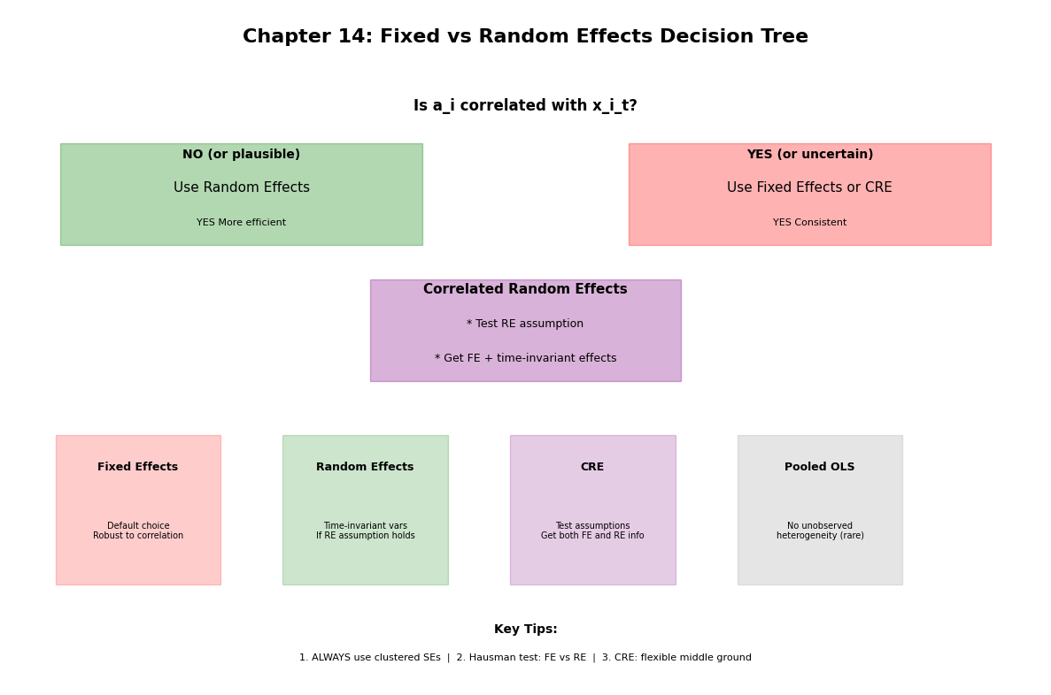
Key Takeaway: The choice between FE, RE, and CRE depends on whether $a_i$ is correlated with the explanatory variables. When in doubt, use FE or CRE for robustness.

Next Steps: Chapter 15 introduces instrumental variables methods for handling endogeneity beyond unobserved heterogeneity.

# Visual summary
fig, ax = plt.subplots(figsize=(12, 8))
ax.axis("off")

# Title
ax.text(
    0.5,
    0.95,
    "Chapter 14: Fixed vs Random Effects Decision Tree",
    ha="center",
    fontsize=16,
    fontweight="bold",
)

# Question 1
ax.text(
    0.5, 0.85, "Is a_i correlated with x_i_t?", ha="center", fontsize=12, fontweight="bold"
)

# Branch: No correlation
ax.add_patch(
    plt.Rectangle((0.05, 0.65), 0.35, 0.15, fill=True, alpha=0.3, color="green")
)
ax.text(0.225, 0.78, "NO (or plausible)", ha="center", fontsize=10, fontweight="bold")
ax.text(0.225, 0.73, "Use Random Effects", ha="center", fontsize=11)
ax.text(0.225, 0.68, "YES More efficient", ha="center", fontsize=8)

# Branch: Yes correlation
ax.add_patch(plt.Rectangle((0.6, 0.65), 0.35, 0.15, fill=True, alpha=0.3, color="red"))
ax.text(0.775, 0.78, "YES (or uncertain)", ha="center", fontsize=10, fontweight="bold")
ax.text(0.775, 0.73, "Use Fixed Effects or CRE", ha="center", fontsize=11)
ax.text(0.775, 0.68, "YES Consistent", ha="center", fontsize=8)

# CRE box
ax.add_patch(
    plt.Rectangle((0.35, 0.45), 0.3, 0.15, fill=True, alpha=0.3, color="purple")
)
ax.text(
    0.5, 0.58, "Correlated Random Effects", ha="center", fontsize=11, fontweight="bold"
)
ax.text(0.5, 0.53, "* Test RE assumption", ha="center", fontsize=9)
ax.text(0.5, 0.48, "* Get FE + time-invariant effects", ha="center", fontsize=9)

# Bottom section: When to use what
methods = ["Fixed Effects", "Random Effects", "CRE", "Pooled OLS"]
uses = [
    "Default choice\nRobust to correlation",
    "Time-invariant vars\nIf RE assumption holds",
    "Test assumptions\nGet both FE and RE info",
    "No unobserved\nheterogeneity (rare)",
]
colors = ["red", "green", "purple", "gray"]

for i, (method, use, color) in enumerate(zip(methods, uses, colors, strict=False)):
    x_pos = 0.125 + i * 0.22
    ax.add_patch(
        plt.Rectangle(
            (x_pos - 0.08, 0.15), 0.16, 0.22, fill=True, alpha=0.2, color=color
        )
    )
    ax.text(x_pos, 0.32, method, ha="center", fontsize=9, fontweight="bold")
    ax.text(x_pos, 0.23, use, ha="center", fontsize=7, va="center")

# Bottom tips
ax.text(0.5, 0.08, "Key Tips:", ha="center", fontsize=10, fontweight="bold")
ax.text(
    0.5,
    0.04,
    "1. ALWAYS use clustered SEs  |  2. Hausman test: FE vs RE  |  3. CRE: flexible middle ground",
    ha="center",
    fontsize=8,
)

plt.tight_layout()
plt.show()